I’ve recently built another closed loop stepper motor board, and this time (with my UROP Yuval’s help building a calibration routine) have a fairly performant commutator for the thing, meaning that it produces good torque with very little wobble. Thanks Yuval!

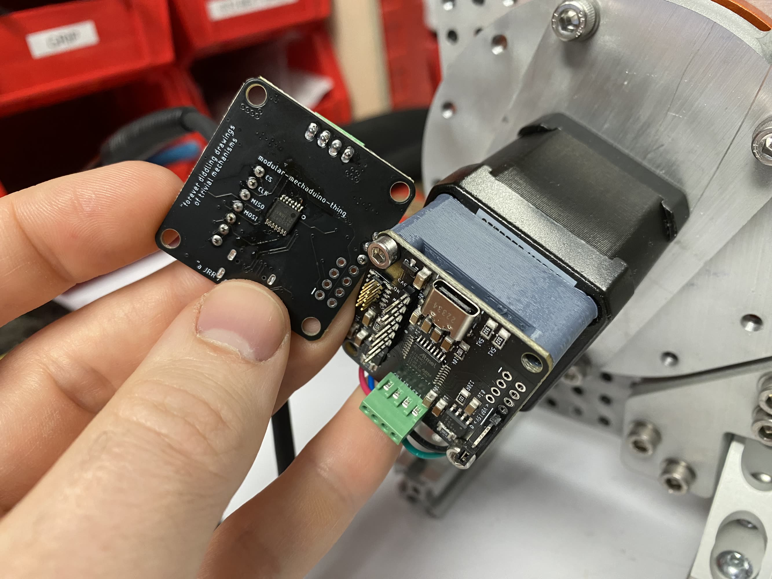
My closed-loop-stepper driver, based basically off of the mechaduino project of yore, uses an AS5047x on-axis magnetic encoder to read the position of a stepper motor shaft. Given a good calibration of the encoder-to-rotor-magnetic-phases relationship, we can use this to commutate the motor like brushless machine.

I’ve also installed this in two test-bed systems, the first of which is a classic cart-pendulum and the second of which is a dynamometer that I built not explicitly for this purpose (I also have a gearbox bone to pick…), but sort of for this purpose.

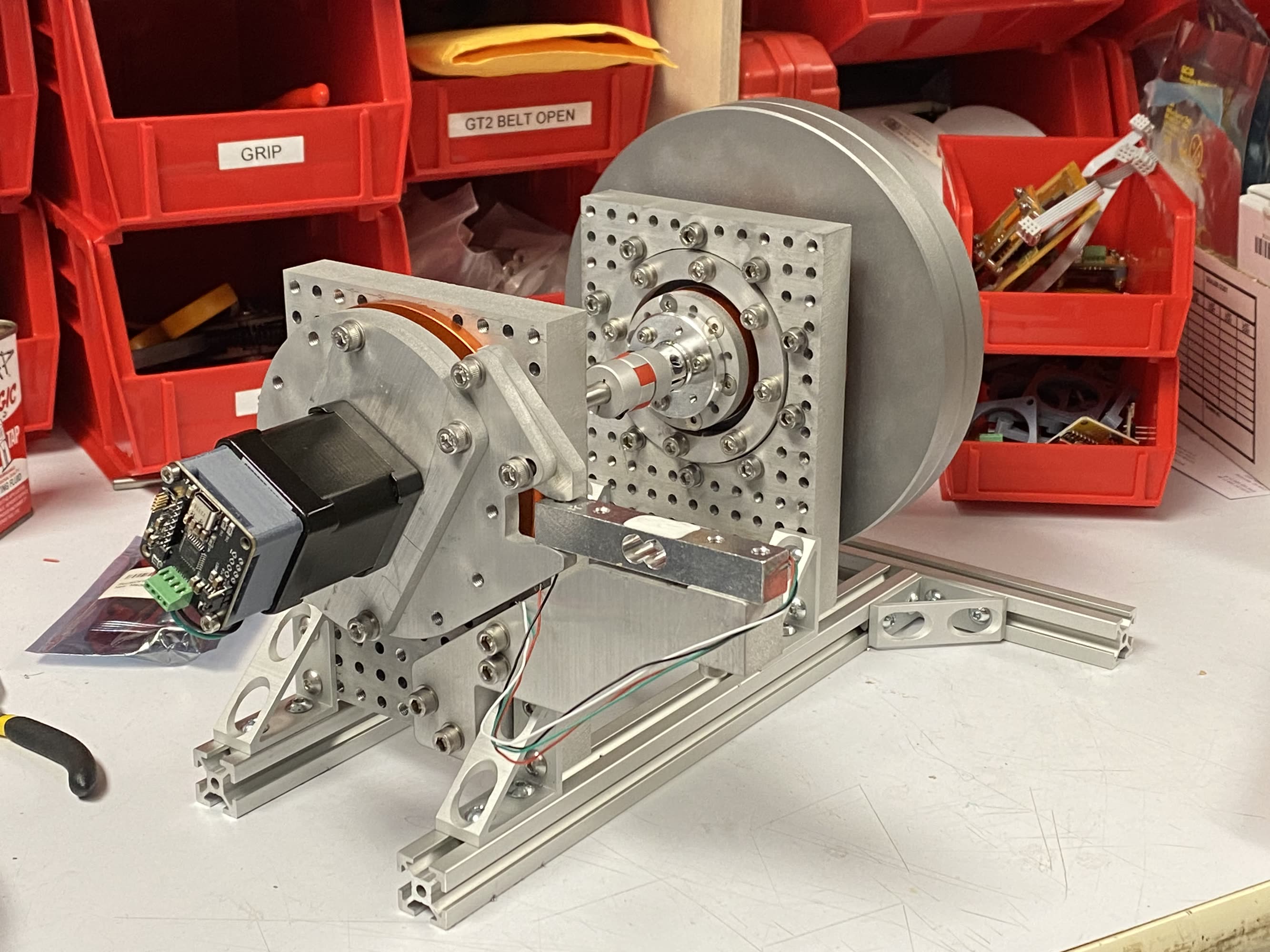
The dynamometer uses a big ol’ inertia (far side) connected to the test motor (left). Both of which are free to rotate (mounted on modular-ish tombstones - the idea being that I can put as many rotary elements in series as I’d like, or i.e. stick a gearbox between a motor and a test load). The motor is constrained in rotation via a loadcell, with which we can read torque. I originally saw this design when David Preiss, a lab mate, built his own dyno.

I also stuck the motor controller on a pendulum-swinging testbed. I later removed the pendulum after realizing the first part of this problem on its own is a PITA.

Looking for Better Systems Descriptions

There are two things I want to explore here: one is using closed-loop controllers (like this) in machine systems to do machine things (you know), and the other is maybe more important: using closed-loop controllers to automatically develop (or fit) computational representations of their performance.

For a little background, you may be familiar with the kind of “classic” motion control trajectories that are deployed in most open-source motion planners (I’m talking about GRBL, Marlin, Smoothieware, and even Klipper) - they look like this:

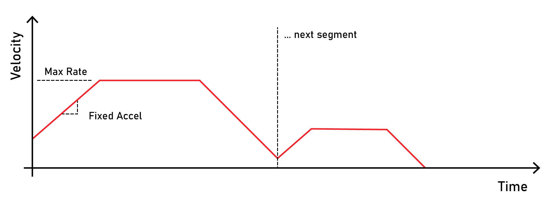
Many motion controllers use simple ‘trapezoidal’ trajectories that describe fixed-acceleration ramps and fixed maximum-velocity limits

We use velocity ramps because instantaneous changes in velocity would produce “infinite” forces on our system, i.e. because \(F = MA\) and our motors can only exert limited torque. Or at least, that’s the abstraction that these trajectories are using (albeit implicitly) to represent the “dynamics” of the motors- and axes- they might be deployed on: that each has one “maximum torque” value and one “maximum speed” limit.

This is a pretty good approximation in many cases, and it continues to serve the open source hardware community pretty well. In particular, trapezoids like this are (1) simple and easily described and interpreted (good for esp. 8-bit firmwares), (2) easily calculated using the kinematic equations, meaning that lookahead planning for a few seconds’ of trajectory can be done in a few ms (or \(\mu s\), depending).

In particular, using dumb representations like this is awesome where systems have to be hand tuned: nobody wants to try writing a state-space matrix for their linear axis by hand, but guessing at maximal accelerations and rates is pretty easy ¹.

However! This robs us of some significant amount of performance, take for example this torque curve:

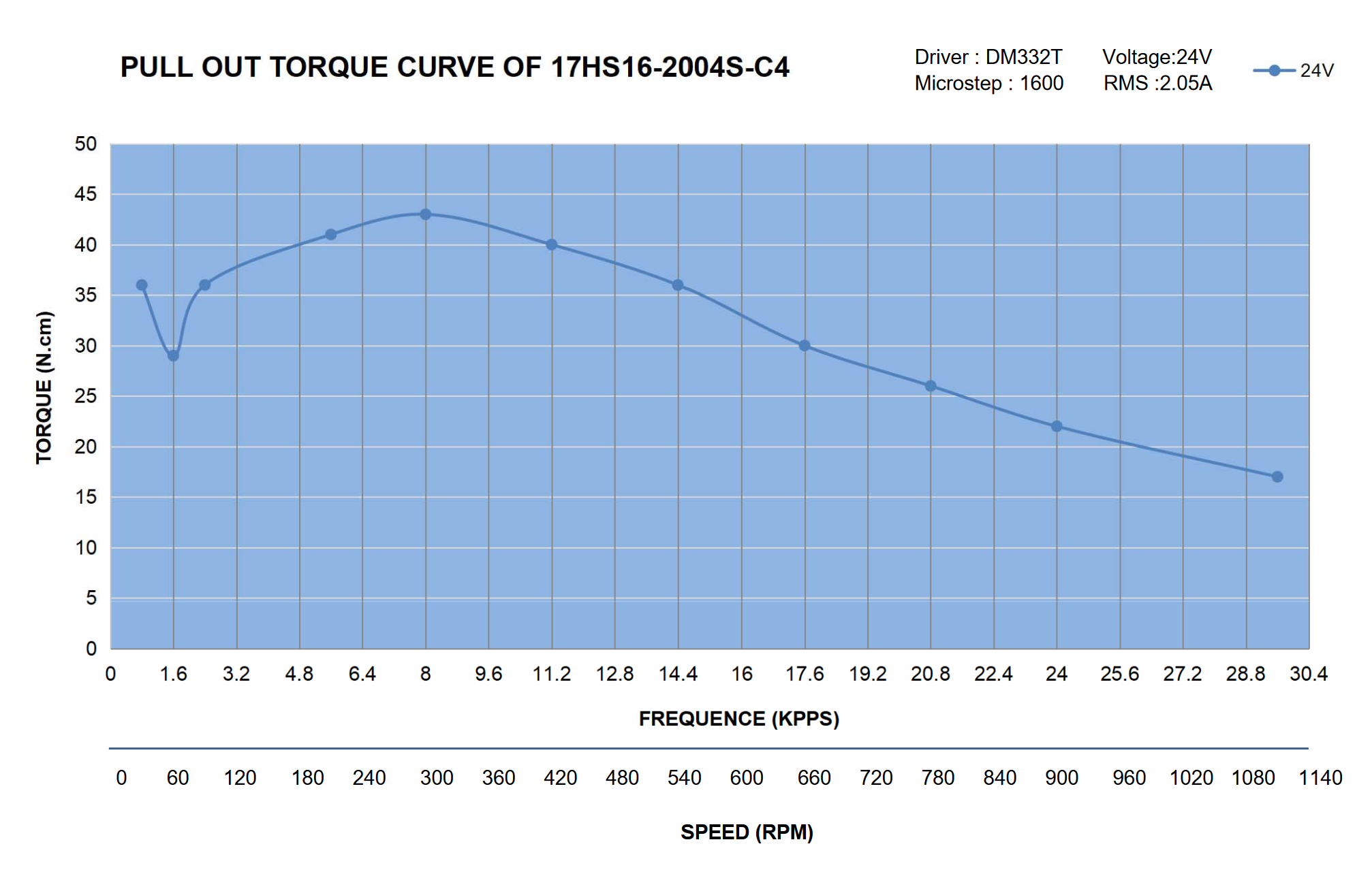
Most motors are spec’d with what is ~ close to a description of the motor as a dynamic system: the torque curve tells us how much torque a motor should produce given it’s current velocity.

Electric motors are more or less all like this: they have lots of torque available “in the low end” (going slow), and it waxes off as speed increases. This has to do mostly with back-emf, but also viscous friction (which increases with speed).

The Payoff of using Better Dynamics Descriptions

With trapezoidal plots, we end up using only some small portion of this torque curve, because we have to set a maximum acceleration that is possible under all speed conditions (not just in the low end). This means we end up implicitly trading off maximal speeds for gruntiness (torque), since we are basically trying to fit a rectangle inside of a curve.

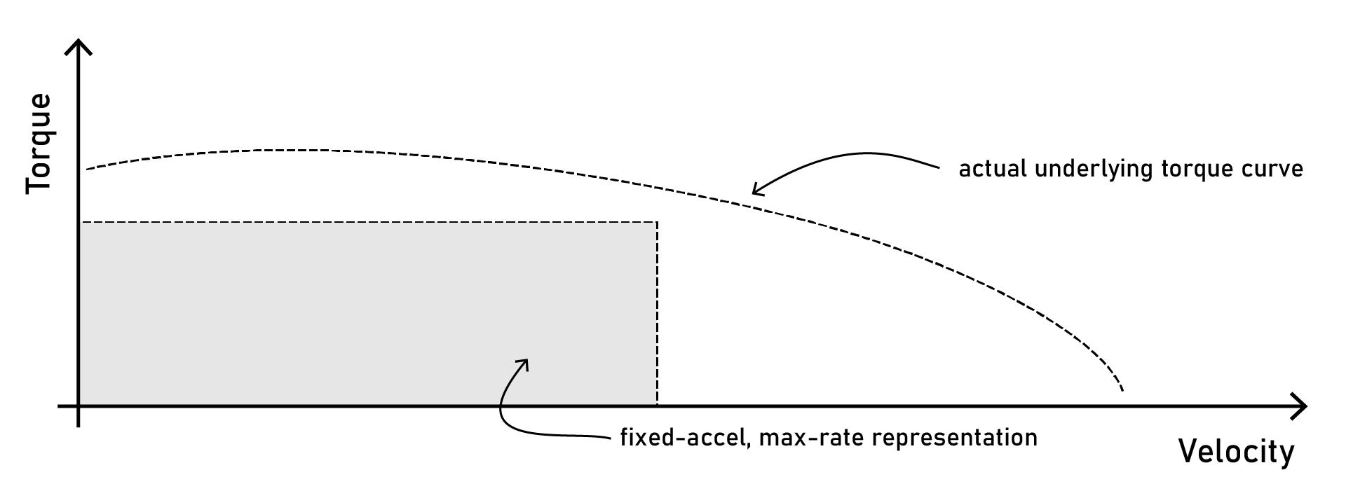
Despite a rich set of underlying dynamics, fixed-acceleration / fixed-rate descriptions only allow operation within a small set of available state.

What’s probably worse about this representation is that everyone is just out there guessing at it - we have no real way, with open loop steppers - to rigorously figure out where our maximal states really are in a system, let alone plan with them and operate throughout them.

So: that’s what this work is about: (1) exploring the manner in which we might articulate dynamics of “typical linear axes” and (2) looking ahead at how motion planners might integrate those descriptions into trajectories that exploit more of our systems’ underlying performance.

Pulling Data

I want to start with looking at some data, because it starts immediately to tell an interesting story. I set-up the dyno, and the motor firwmare, and basically tried to get the thing to sweep through lots of different velocity-and-acceleration states. That is to say, I swung the inertia back-and-forth with varying force.

To gather dyno data, I just apply voltage to the motor in an alternating, decreasing pattern. This does a decent job of covering many likely places in the system’s state space.

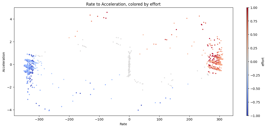
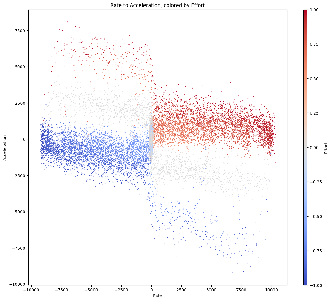
From this I get a whack of time-series data that I can organize into a torque-curve-looking-thing, a kind of phase-space plot.

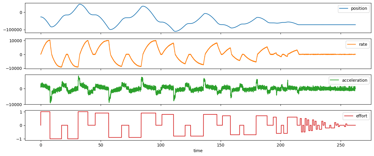
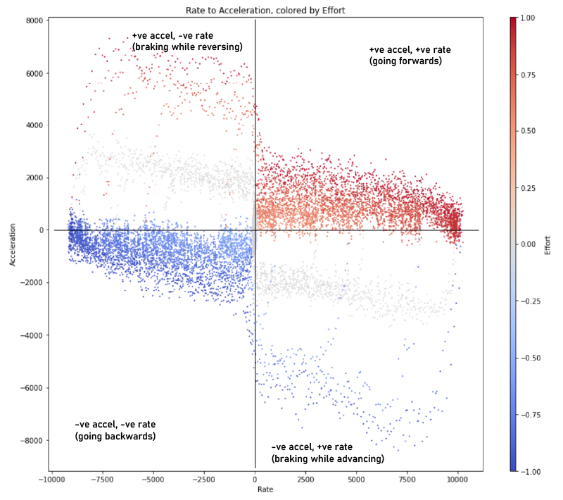
Time series data (above) can be orgnized into a phase-space plot that’s somewhat analogous to a torque curve: it plots observed accelerations across various speeds. This plot would be enough to completely describe a system with no third-order dynamics (i.e where instantaneous changes to acceleration were possible), but most of our motors have observable delays in torque generation since current cannot be produced instantaneously.

Braking Acceleration Can Far Exceed Startup Accleration

This is the first clear observation we get from the data: our systems should be exploiting the assymmetry that arises from braking force… quadrants 2 and 4 show deceleration that combines motor forces with the systems’ natural friction-generated forces for about 3x “performance” over straight acceleration (where velocity and acceleration vectors are aligned).

Linear Axis Data Gather

I also got a linear axis together and, using the same motor, tried to collect some useful data there:

Data gathering on the linear axis by sweeping back-and-forth between virtual endpoints.

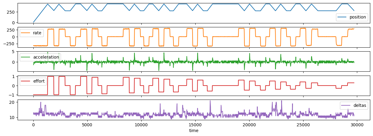
A similar data-set from a testbed linear axis, including a trace of deltas - how long (in ms) we wait between each respective sample.

These data are OK, but (largely due to my sampling speed) we miss most of the interesting points… the constant-velocity segments here dominate the time-series, and the turnaround events last only a few ms - perhaps 250ms on the long side. Since our sampling frequency is only around ~ 15ms (I’ve written a pretty naive data-gather routine), the state space that we’re interested in is pretty sparse.

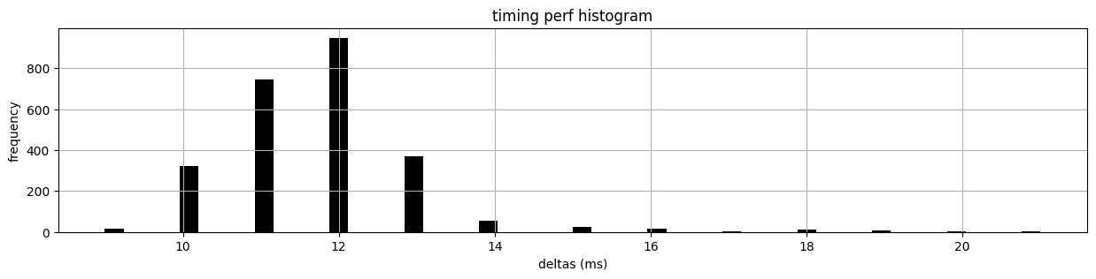
Bad timing performance on the data-gather side hobbles our ability to inspect the linear axis testbed properly. This should be easily remedied in the future with some code upgrades - that should also allow us to build fixed-interval timeseries (these are all polling, and so have varied intervals).

How to Model These Systems

So - we have seen some data, but what are we actually expecting to see, if we model this stuff? I tried working through the motor- and inertial ODEs… s/o to this video for a refresher.

Motor Equations

Given a motor, we have Kirchov’s votage law (sum of all voltages in our loop is equal to zero):

Where \(V\) is voltage applied and voltage due to back-emf, \(I\) is the current travelling through the loop, \(R\) is the motor’s coil resistance, \(L\) is the motor’s inductance (attached to the 1st derivative of current \(\dot{I}\)).

Inertia Stuff

We also have an inertia and a damper (friction, as a proportion \(k_d\) of our speed), say our inertia has an inertia \(J\) and velocity \(\Theta\) and acceleration \(\dot{\Theta}\) - we have also some torque being inserted into that system from the motor that we’ll call \(Q_m\) - which we can make another statement about our acceleration:

Linkages

Now we need to link the electrical machine to the rest of the thing, so we have \(k_t\) - a torque constant:

We also have our back emf constant \(k_{emf}\)

The Hookup

So we roughly have one equation for the motor voltage:

And one for the inertial damper side:

Integrating

We’re going to drive our system at the bottom with \(V_{app}\) so we’ll want to see \(\dot{I}\) as a function of that:

We’ll also want to be able to get \(\ddot{\Theta}\), that’s here:

ODEs in Python

This was the part that I never really clocked about “differential equations” (which sound scary) - they’re really just nice articulations of how systems evolve… or, especially in simple cases, are tiny integrators for computer simulators… so, the programmers among us may have a better time if we describe the system a-la:

# our system params 
r = 4.0 # resistance of the motor coil (ohms ?)
l = 2.2 # inductance of the motor coil (henries ?)
j = 1.0 # rotor inertia (kg/m^3, or sth?)
kd = 0.5 # damping factor (...)
kt = 1.0 # torque constant (...)
kemf = 1.0 # rippums to voltage linkage (...)

# get the change in current (~ roughly equiv to change in accel)
def calc_i_dot(v_app, i, r, l, kemf, theta_dot):
    return (v_app - i * r - kemf * theta_dot) / l

# get the acceleration: current... plus some velocity-dependent damping 
def calc_theta_ddot(i, kt, theta_dot, kd, j):
    return (kt * i - kd * theta_dot) / j 

# then we can integrate through time... here's a function that 
# returns new system states, given previous states and some time-step 
def integrate(v_app, i, theta_dot, theta, delta_t):
    # first we calc delta-i given v_app, 
    i_dot = calc_i_dot(v_app, i, r, l, kemf, theta_dot)
    # we use that to integrate i, 
    i += i_dot * delta_t 
    # i is related to acceleration like-so, 
    theta_ddot = calc_theta_ddot(i, kt, theta_dot, kd, j)
    # we use that to integrate theta_dot and theta, 
    theta_dot += theta_ddot * delta_t 
    # and thru theta, 
    theta += theta_dot * delta_t 
    # and we return out whole-ass state vector, w/o the lowest state:
    return i, theta_ddot, theta_dot, theta 

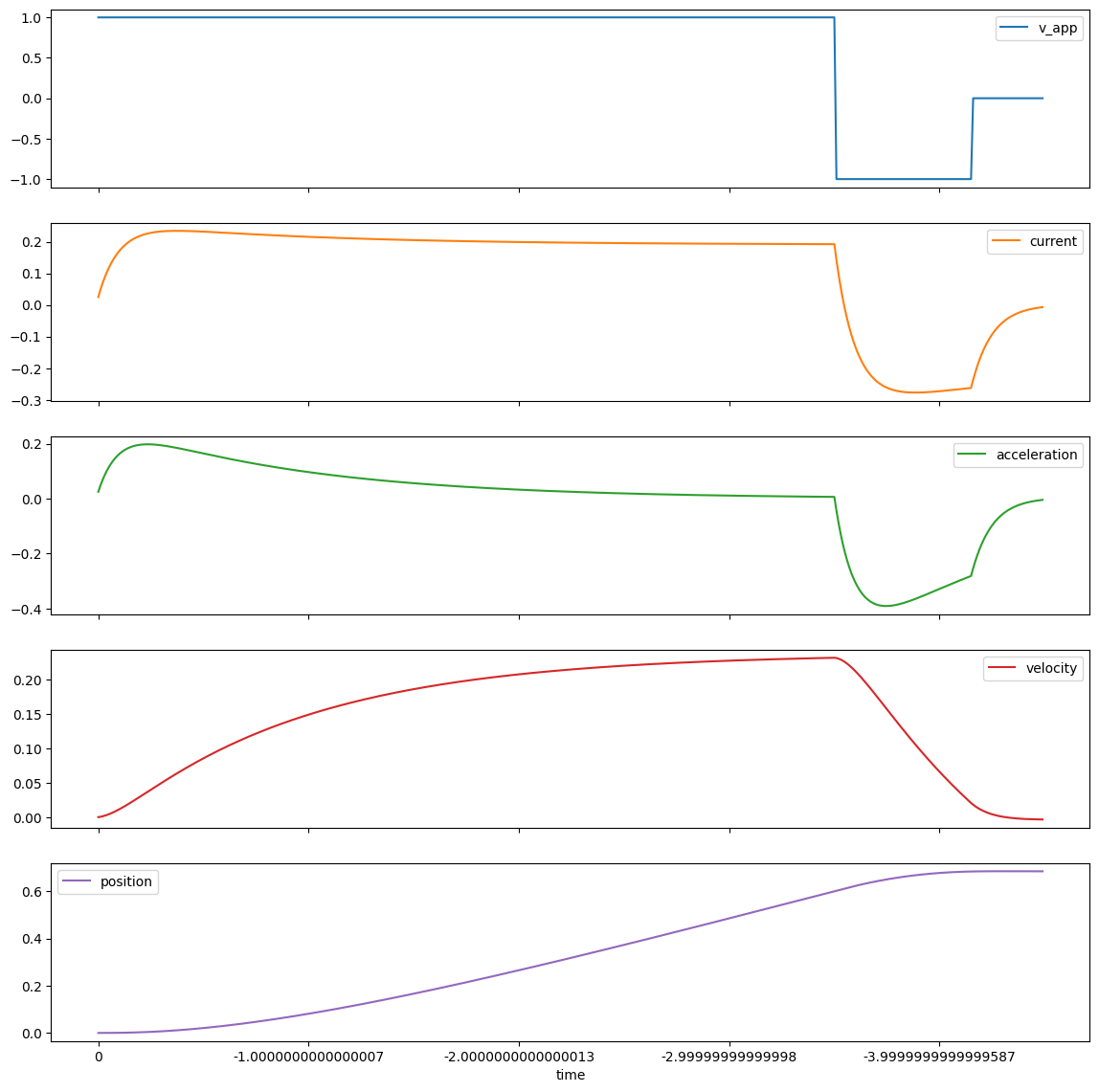
Then we can operate that system similar to the way we were operating our real-world objects, basically swinging them back and forth, trying to cover lots of the state space:

df = pd.DataFrame(columns=['time', 'v_app', 'current', 'acceleration', 'velocity', 'position'])

#start with state vector as
i = 0 
theta_ddot = 0 
theta_dot = 0 
theta = 0 

# step as
timeStep = 0.01
time = 0 

def run_until_steady(effort):
    global df, time, i, theta_ddot, theta_dot, theta
    plotulo = 0
    while True:
        # plot runtime... 
        plotulo = plotulo + 1 
        if plotulo % 10 == 0:
            clear_output(wait=True)
            print('{:.3f}, {:.1f}, {:.3f}'.format(time, effort, theta_ddot))        
        # integrate and stash, 
        i, theta_ddot, theta_dot, theta = integrate(effort, i, theta_dot, theta, timeStep)
        df = pd.concat([df, pd.DataFrame({
            'time': [time], 
            'v_app': [effort], 
            'current': [i],
            'acceleration': [theta_ddot],
            'velocity': [theta_dot],
            'position': [theta]
        })], ignore_index=True)
        # add time 
        time += timeStep 
        # check if steady 
        if(abs(theta_ddot) < 0.001):
            break

def measurement_cycle(effort):
    run_until_steady(effort)
    run_until_steady(-effort)
    run_until_steady(0)
    run_until_steady(-effort)
    run_until_steady(effort)
    run_until_steady(0)

run_voltage = 1 

while True:
    if run_voltage < 0.1:
        break
    measurement_cycle(run_voltage)
    run_voltage = run_voltage - 0.2

print('... done')

This generates more time-series data!

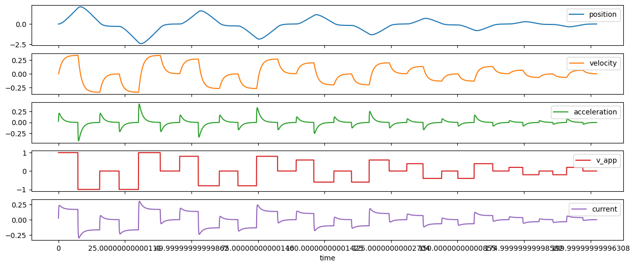
A similar data-set from a testbed linear axis, including a trace of deltas - how long (in ms) we wait between each respective sample.

(Qualitatively) Matching ODEs to Dyno Data

Fitting actual-values is one thing, but we want first to check if we can get a qualitative fit (same shapes)…

Dyno Data in Phase Space	ODE Data in Phase Space

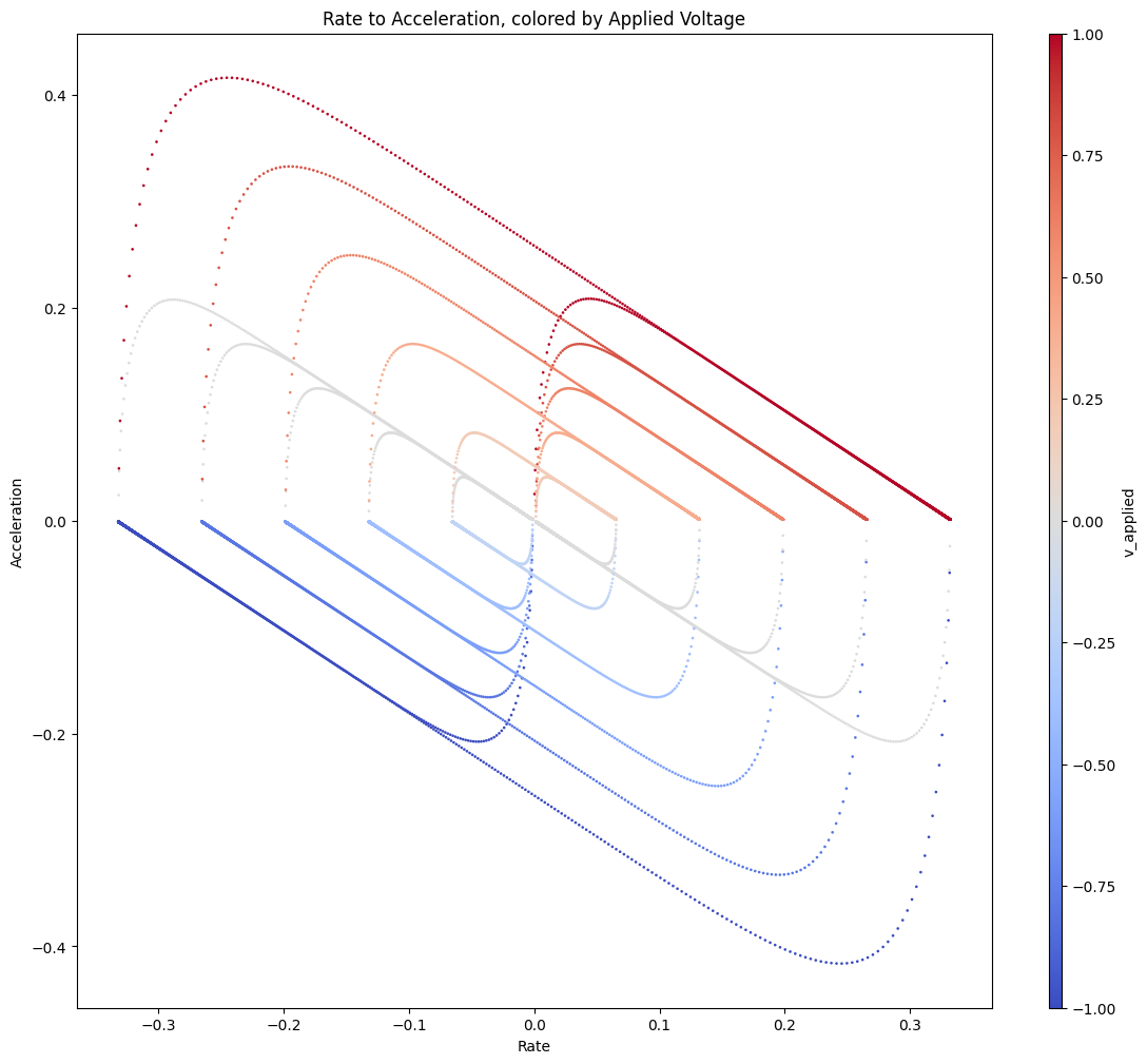These don’t seem terribly mismatched (and I will note that the ODEs I described earlier are the canonical set for this type of system) but there’s clearly something missing around the origin that I don’t think we would get away with ignoring. I originally figured it had to do with one of these nonlinear friction models (which I should anyways try to include in these models), but it actually turns out to be better fit with assymetric torque.

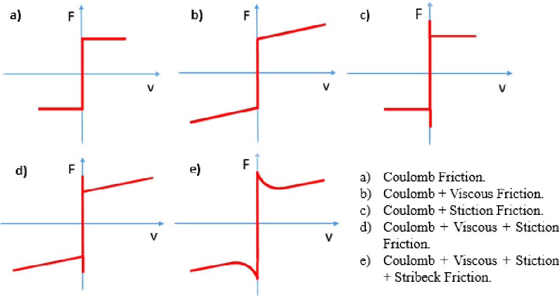
A selection of nonlinear friction models, from Nonlinear Friction Identification of A Linear Voice Coil DC Motor

To implement “assymetric torque” we just check signs of velocities vs. current:

def calc_theta_ddot(i, kt, theta_dot, kd, j):
    # we have, I suspect, an assymmetry in the motor's ability to 
    # sink (brake) vs. source (pull-out) current 
    if (i > 0 and theta_dot > 0) or (i < 0 and theta_dot < 0):
        # torque constant for accel-in-dir-of-speed, 
        kt = 1.0
    else:
        # torque constant for accel-in-reverse-of-speed:
        # i.e. regen / braking: 
        kt = 2.0
    return (kt * i - kd * theta_dot) / j 

This results in something a little closer…

Dyno Data in Phase Space	ODE Data in Phase Space

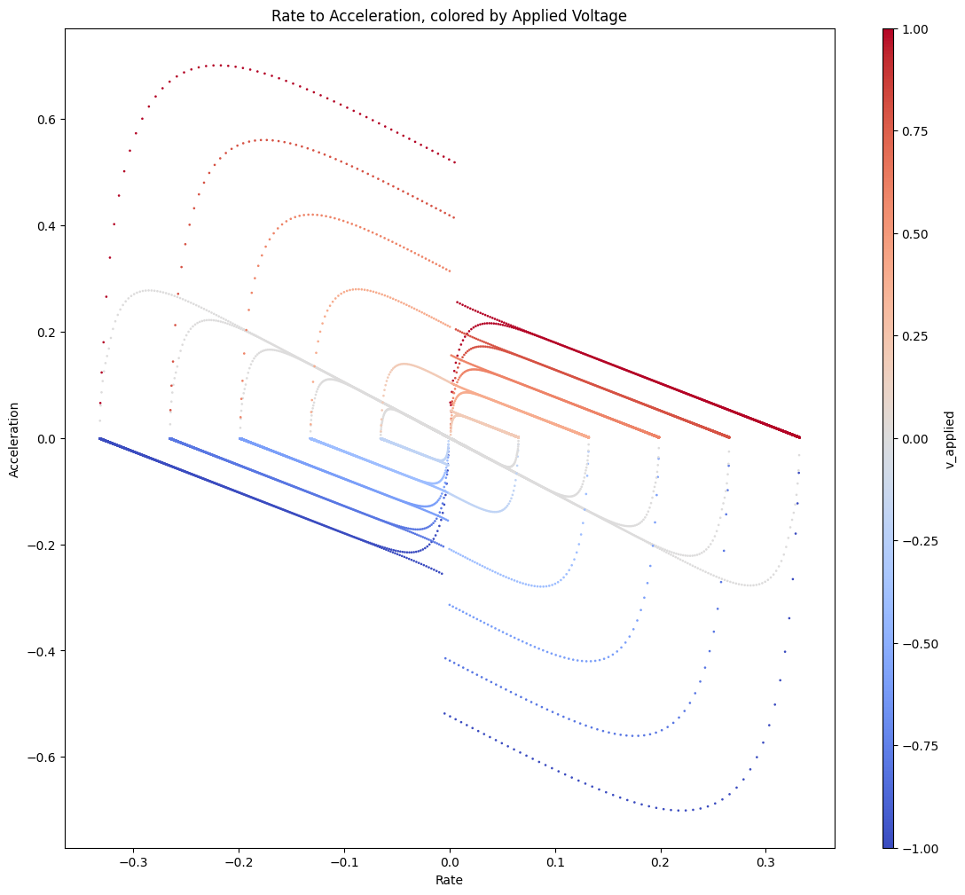It might even be better to do this in the next order down, to preserve the no-instantaneous-current-changes… in any case, I’ll have to suss that out in the future. I think the phenomenology here is basically that… the h-bridges in the motor driver have a better time sinking (fast decaying) current than they do have of sourcing it. Kind of like in an automobile… it’s easier to hit the brakes and turn energy into heat than it is to loose new energy into the system.

State Evolution and Vector Field Representations

Now, I’ve generated a few fits for the data using DMDc and SINDYc, but I don’t totally understand those yet so I’m going to hold off on reporting on them. Next rambling post…

What I do think that I have understood at this point, and what this whole post is getting towards, is how to best represent “these systems” - as in, dynamical stuff. In a way that makes sense to a caveman / mostly-mechanic’s-blood type like myself.

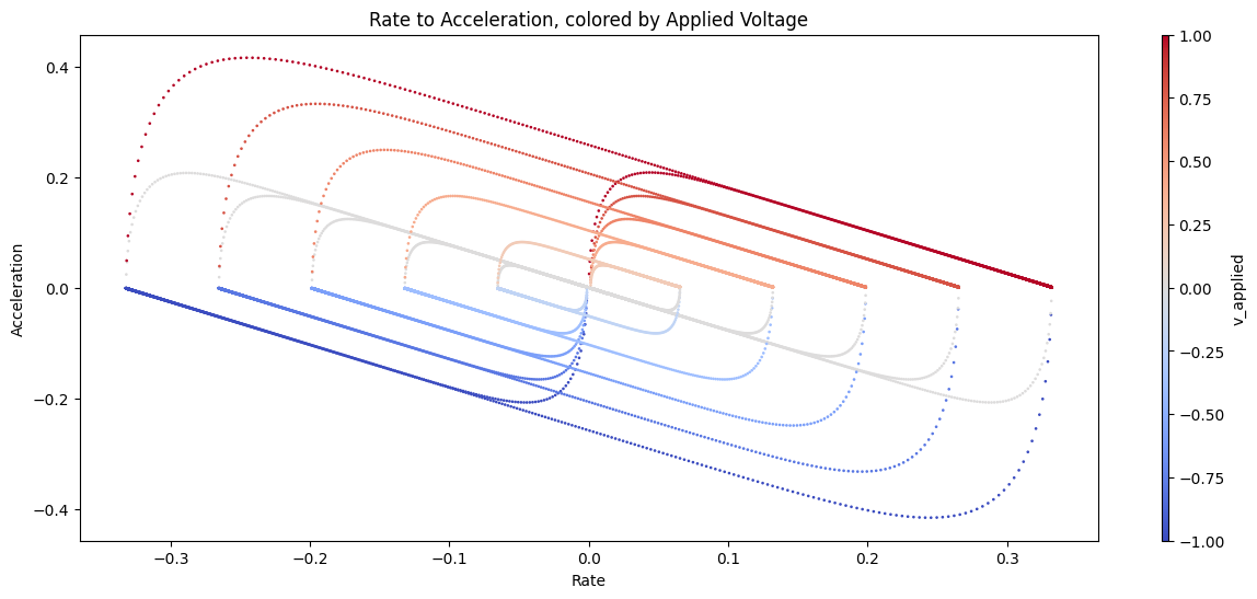
I’ve been on about the phase-space plots, that map acceleration as (roughly) a function of velocity. These are awesome, but what’s better is a vector field, that maps how a system, from any state, moves towards other states.

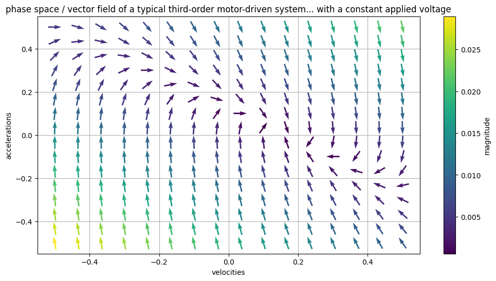
Vector fields can represent dynamical systems really concisely: they point from any state, to the likely next state. In this plot, we see how accelerations and velocities evolve under a fixed applied voltage. There’s a stable point around [0.2, 0] that the system falls towards: a maximal velocity given the fixed effort.

These are rad, and make it possible to express how the system behaves without any direct relation to a particular time series. However, by tracing paths through them, we can imagine how a time series would evolve.

The vector field I’m showing above has a fixed applied voltage, i.e. a controller that isn’t doing anything. Of course our controllers are interested in changing how a system evolves over time, so it’s useful of thinking of these plots as kind of… environments we can alter with our controllers, to drive systems to certain states.

You can slide the knob here to adjust the applied voltage to the system, and see how the vector field changes…

One way to think of these is like a big tilting-marble-maze, you know the ones:

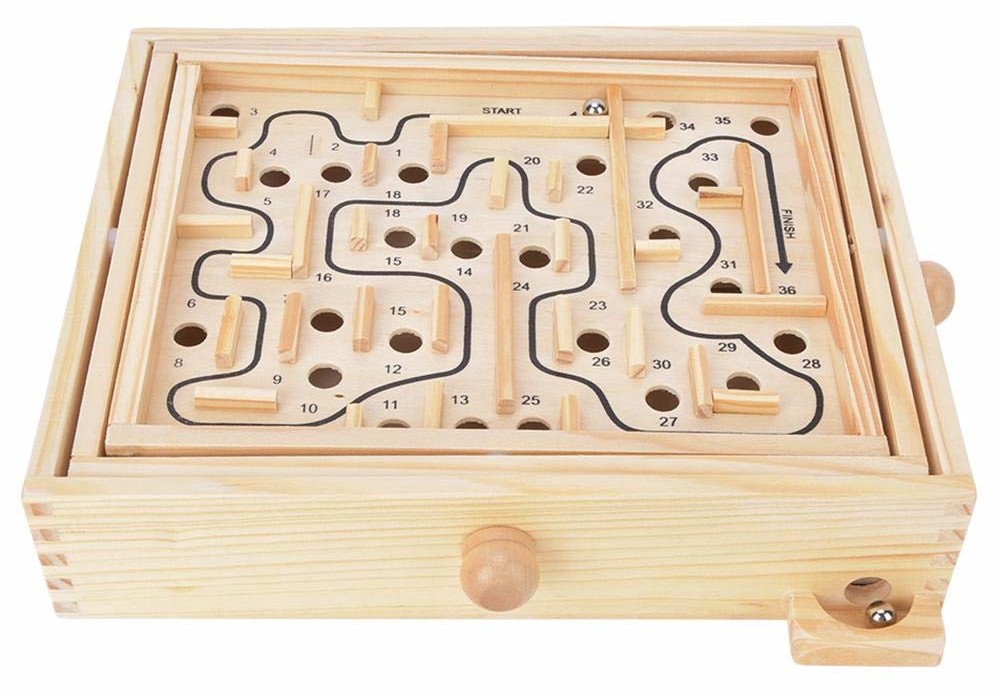
But our ‘knobs’ (here the v_app / applied voltage - which, fwiw, controls-folks normally label as \(u\) or a vector thereof) have a more complex mapping to the slope that the ball rolls along. So - in order to do any control - we need to understand this mapping.

Another way to think of these things is just as integrators. Given a vector field, and some initial position, we can pretty easily trace the contour of how our system is going to evolve over time. One result of that, which I suspect is going to be useful for future me, is that we will be able to use vector fields to represent almost any description of a dynamical system - whether we pick DMDc, SINDYc, neural-net or simple ODE-fit representations.

Mathematical Language for Evolving Systems

I started this work trying to understand how to fit a model to the data that my dyno and linear axis produce, but the work ended up serving as a refresher for me on dynamics systems in general. My main frustration throughout the spiral was in figuring how to represent the things - I wanted to see my ODEs (for example) on the same terms as I could express my data, to see matches, or fits.

The vector field ended up being an awesome way to visualize this, but it seems to me that the canonical language of controls systems is basically the same representation, that is, state space models in this form:

Are basically just integrators - i.e. they tell us how our state vector \(x\) should be updated (i.e. what are the changes in \(x\), the \(\dot{x}\)) - for any given state. The update is described with the \(A\) matrix that acts “just on the states” (i.e. has no relation to control inputs) and the \(B\) matrix is multiplied with \(u\) - i.e. our control vector (in these examples, and in many others, that’s just one number: normally some voltage, since we can write those straight out of microcontrollers). Meaning the \(B\) matrix describes how our controllers can interact with systems.

There is an equally (perhaps even more-so) salient discrete time representation:

That is, the A and B matrices work together to simply predict the next time-step, given the states at the last time-step. This formulation is one-hundred percent identical to a typical digital integrator, or simulation, of these dynamical systems.

What Have we Learned?

So, I’m going to stop here and return next time to look at various fits of the data. Hopefully the third post (in a triad?) would implement those fits, i.e. swing the pendulum up, optimizing trajectories, etc.

Data Gathering Lessons

Here, I have not much to say other than: having clean, high-time-resolution data seems really important. I will spend some time engineering better perf, doing i.e. bulk transport of multiple time-stamps, better data framing, etc.

Vector Fields / System Evolution is the Right Framework for Representation

I love these fields: they’re intuitive, kind of nifty, and will work to describe almost-any model in the same terms… what’s more, we can probably use them even to plot raw data, so that we can visually inspect model fits. Rad.

Model-Informed Lookahead Might Drastically Improve Machine Performance

I guess this isn’t too surprising, but looking at that accel-vs-velocity plot from the dyno was shocking: mostly w/r/t how much unexploited assymetry exists between braking- and launching- acceleration.

Nonlinearities Abound in our Motor Controller

The assymetry above I believe is due in two-parts: one helping of friction (probably also nonlinear), and one helping of sourcing (low) vs. sinking (high) current capability in the motor drivers. Fitting those… might be tricky, so, we will see how i.e. SINDYc or Neural Nets do, or, I will author some more-complete ODEs.

What’s Next?

Like I think I alluded to, I want to follow this (1) up with (2) testing various model fits and then (3) implementing closed-loop controllers or / and optimal trajectories through one DOF. (4) would go to multi-dof systems and things like FDM extruders (that have actually nasty nonlinearities).

What Optimal Trajectories Might Look Like

I want to throw this down here for now, though, since we started by looking at trapezoidal trajectories.

Although I wrote the control time-series for this by-hand, it shows us what really-optimal lookahead trajectories might look like, given motor models like those explored in this write-up.

Solving these trajectories in the general sense is straight up constrained optimization, and Quentin has taken a stab at it recently, with a really cool implementation. We’re actively working on this, so I am excited to see where it… takes us… (get it?) in the future.

How to Encapsulate and Transmit Trajectories

Implicit in all of this is that we’re solving for trajectories using i.e. laptop-sized computers that can run python with scipy / numpy / etc. Once we write optimized trajectories, we’ll need to get them into motors so that they can be followed / executed.

We especially would like a version of this system where we can write trajectories into open-loop motors, having learned what “typical” systems look like, i.e. using closed-loop motors on a testbed machine, learning its dynamics, saving models, and using those to generate trajectories for deployed machines that use cheaper, simpler, and more robust open-loop controllers - but still feed those controllers optimal trajectories based on the underlying dynamics (with some safety factor of course).

Or, we would want to mix open- and closed-loop hardware together in modular machine systems… in either case, we want a compressible trajectory.

For this, we’re looking at a final step of hermite spline fits, basically delivering to groups of motors time-delineated functions that they can intermittently check against their actual positions to i.e. update stepper state-machines or position targets for simple feed-back controllers (PID), or even use as trajectory sources for a few samples’ worth of MPC control.

Towards Fast AF Machines!

This feels like the first real start towards implementing really high-quality motion control across our modular machines. I suspect that there is lots left to learn, and I hope that I can keep up with this exercise of sharing new (to me) knowledge once I’m through with each step.

TTFN,
Jake

Footnotes