What feels like ages ago when we were both at the CBA, Sam Calisch pointed out to me that it’s possible to control a stepper motor as if it were a brushless motor, using field oriented control, aka FOC - everyone’s favourite motor control algorithm. This was an exciting idea and I quickly built a circuit to carry it out and I made a decent pass on the project back in 2021 although I never managed to completely integrate it into a motion controller.

Since then I have some new hardware with better current measurement, and a better idea about how to integrate the thing with the rest of the motion control problem, so I am back to learn again.

In particular, I want to learn how to do this across generalizeable hardware - i.e. slap a controller onto whatever motor is lying around and transform it into a high performance servo. To do this, I need to understand and implement FOC, and then use the controller hardware to learn enough about whichever particular motor it finds itself on in order to control it successfully. In this post, I mostly accomplish the first task, and learn lots about the second.

The result of this effort: a NEMA14 stepper motor in closed-loop position mode, reporting torque in real-world units, using a motor model that was (partially) learned using the motor itself.

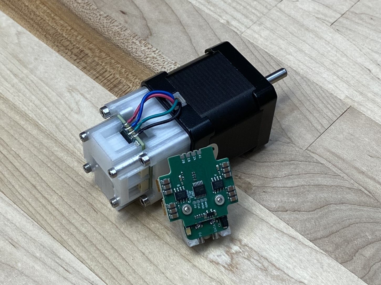
The closed-loop stepper board, and one of the same mounted on a NEMA17 motor.

Whether or not this is a good idea has been the subject of many a heated debate in the dungeon basement of the CBA. Proponents argue that steppers might have more low end torque than ‘normal’ brushless (BLDC) motors - probably due to their high pole count. This seems likely to me, but only in an intuitive way. It seems that they are almost definitely less power dense than BLDCs, but again all I can stand on there is intuition… steppers are built with a lot more magnet steel than seems necessary. Hopefully I will find time to look into (and write up) some more fundamental motor physics that would explain these trade-offs, but in practice I think they are often more subject to the availability of components for our project than first principles physics, and stepper motors are downright ubiquitous - and downright cheap. Hence the almost-any-motor framing for the project.

I have to make a shout-out to the mechaduino project, which is the first implementation I saw - I think there are many such projects out there, and I know this is not terribly novel of me. FWIW, I suspect that the real lack of closed-loop in open-source has to do more with the systems we use to integrate motors with motion controllers (and tune servo loops) than the availability of motor controllers themselves. I have done lots of work building higher-level motion controllers / planners (synchronization, look-ahead, and even model-predictive motion lately), but I wanted to come back to the low level and see how that might all connect to i.e. position PIDs.

So, in this post:

• a brief explainer on FOC and its relevance / application to steppers
• a tour through the hardware and some of the low-level controller components
  • ADC aligned sampling
  • current control in rotating reference frames
  • encoder calibrations
  • a simple position / velocity / acceleration observer
• some motor data collection and modeling to find (kt, ke, kd)
• learning how to use the motor as a sensor even when we are running open loop
• some notes on integration with motion systems

Stepper FOC vs. Brushless Direct Current (BLDC) Motors

Electric motor architectures are proliferating, especially due to interest in EVs - but all share the same principle: the rotor has a magnetic field - normally provided by permanent magnets made of those geopolitically sensitive rare earth metals - and the stator has electromagnet windings. We then use a computer to switch current through the stator windings, so that we can “point” the stator’s magnetic field in whichever direction we would like.

In all cases, what we want to do is drive the stator’s magnetic field so that it is 90’ out of phase (left or right) from the rotor’s magnetic field. Since the rotor’s field wants to align with the stator, the 90’ phase advance effectively pulls the rotor in that direction. Moving the stator’s field so that it advances ahead of the rotor’s field is known as commutation, and we call the reference frame that rotates with the rotor the dq frame, with a direct axis that is aligned with the rotor’s magnetic field, and a quadrature axis that is 90’ offset from that axis.

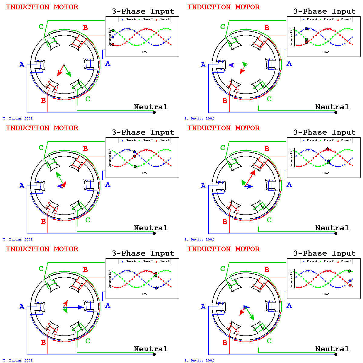
In a motor with three phases, like BLDC motors or most induction motors, we have three magnet windings in the stator that make up a kind of set of basis vectors. By varying the current on these three windings, we can effectively point a current vector within in the stator.

The best explainer on stepper motor operation that I could find.

Even though they are fundamentally the same as any other motor, steppers can be confusing since they are ‘hybrid’ architectures, combining normal permanent magnet motor design patterns with ‘reluctance.’ This basically means the field generated by the permanent is carefully guided through patterns in the rotor’s laminations. If you’re unfamiliar, the video above is the best way to learn.

When we’re doing control, it’s almost better to not think about those finer details. What we really want to know is that the stepper has 50 electrical rotations for every mechanical rotation - that is, every time we swing the shaft around once [0-2PI] radians we rotate the magnetic field around inside the stator fifty times. There are four ‘full steps’ in each full rotation of the electrical phase, hence 200 ‘steps’ in a motor.

The image below via allaboutcircuits shows an effective way to think about a stepper motor, for control purposes. We have two windings - one ‘up and down’ (the ‘B’ winding) and one ‘side to side’ (the ‘A’ winding) (sometimes X and Y, depending on the parlance).

If we only drive current from left to right on the horizontal winding, we are putting all of our current at zero degrees. If we only drive current ‘up’ on the vertical winding, we are putting current at ninety degrees… and so on: right to left = 180 degs, down = 270 degs. We combine components of these to drive current at whichever angle we would like.

We can effectively think of stepper motor stators as an electromagnet with two windings: one pair side-to-side (A) and one up-down (B). These are basically basis vectors A, B (or X, Y depending on who you are asking) that we can use to control the direction and amplitude of the magnetic field within our stator.

So, besides the particular layout of the hardware, FOC applies just about identically to the stepper. In fact the algorithm is smaller, since our component vectors are a simple orthagonal set (rather than the 120’ separated phases in a BLDC). That said, FOC in a stepper probably needs to commutate faster than in a BLDC (since the phases are so tightly packed), and steppers tend to have higher inductance, meaning we might want more voltage to swing the things around.

The Hardware

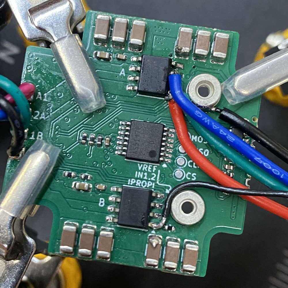
My FOC-stepper board, with current sensing and PWM pins bodged out for debugging. Microcontroller (SAMD51) and an interface for comms is on the other side. It’s a busy fit on a NEMA11, but well sized for NEMA14s, and can probably drive up to NEMA23 windings.

Some specs for you:

MCU: SAMD51J19A, 120 ~ 200MHz, ARM-M4F
Encoder: AS5047P, 14 bit, on-axis magnetic
Drive: 2x DRV8251A, 4.5-50v, 4.1A peak, 450mOhm, current sense out
I2C Port
Fan Port
Motor Thermistor Plug
Limit Switch Plug

The board is part of a family that I am calling knuckles - that share physical link hardware with a swappable PHY spec, TBD on releasing that but it basically means that we can put whatever connectivity we want onto this thing: USB + USB PD for development is pretty handy, I also have an RS-485 adapter, and should develop CAN and BLE versions, etc.

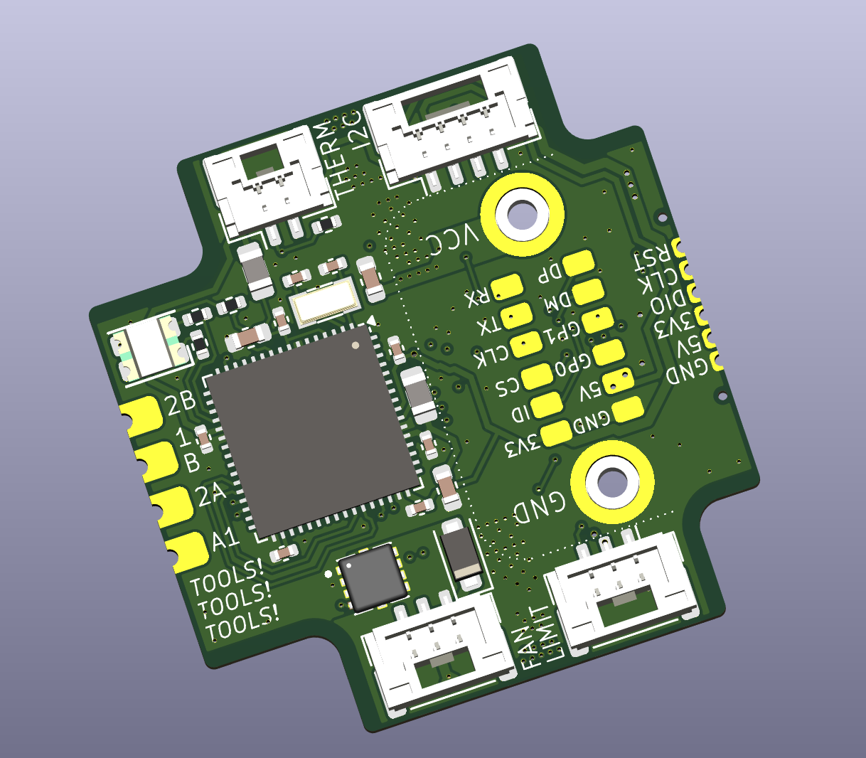
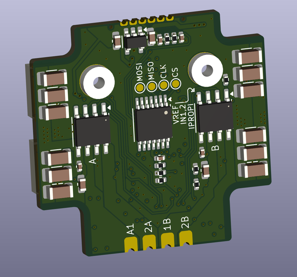
Front and Back, from KiCAD. The group of 12 labelled pads is the interface for a modular PHY layer that I am developing.

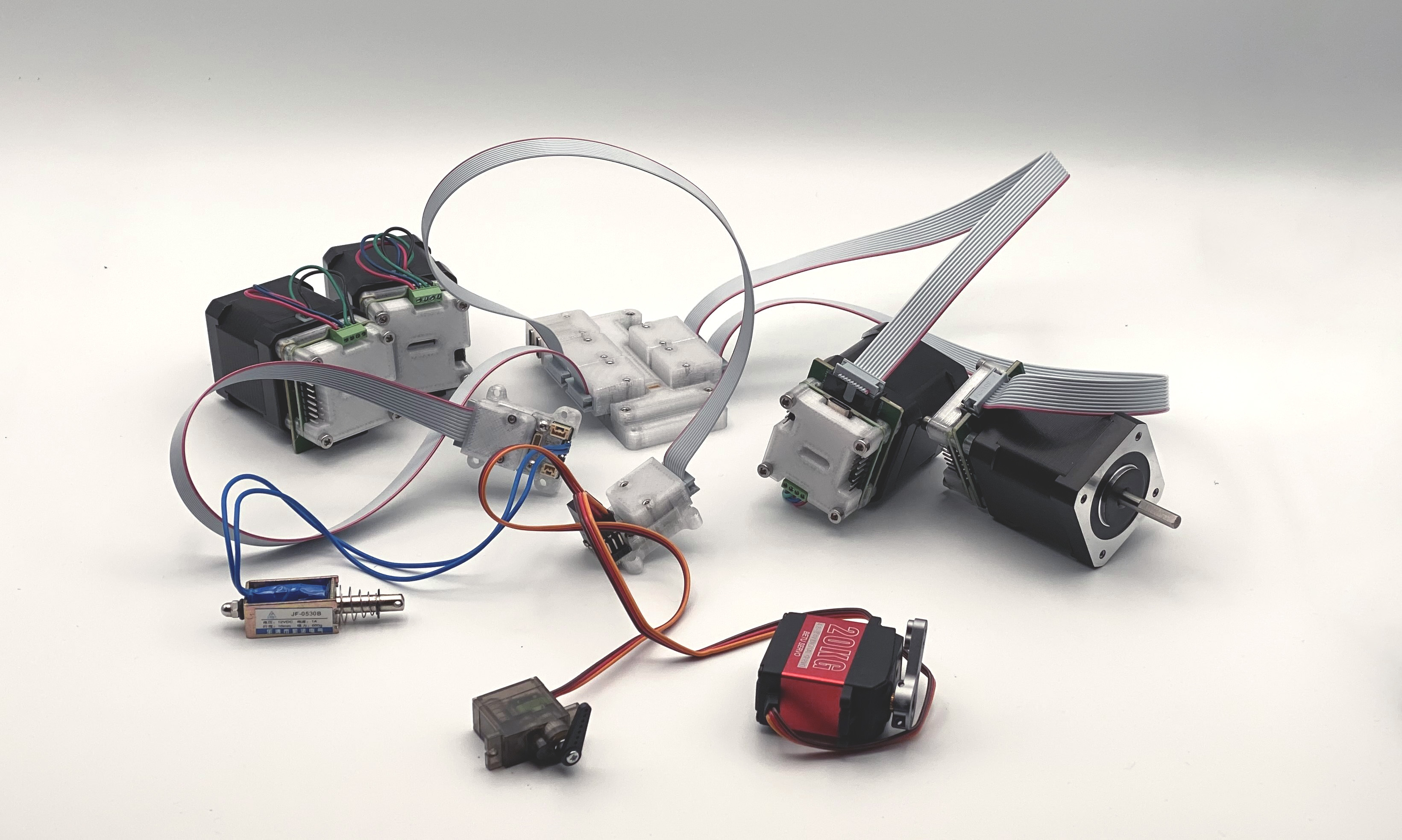
Some of of the’knuckles’ family of modular circuits, showing also the small embedded message passing and power distribution device (top center).

This fits ish on a NEMA11, and fits well on NEMA14 up to 23, where I suspect that the drivers would start to be a little bit heat challenged. I did put a small fan driver stage on the board for active cooling, and with the right enclosure / heatsink I think NEMA23 is totally manageable - at least the shorties.

TODO: pics of the circuit mounted on motors !

The board is four-layers, the two internal layers were aspirationally all GND plane but I had to cheat a little and route some lines under the microcontroller. This layout was tricky because I was really trying to pinch the thing onto a NEMA11, but I think I worked it out well. I do love a good routing challenge even though it normally takes me ~ four days instead of the two that I budget.

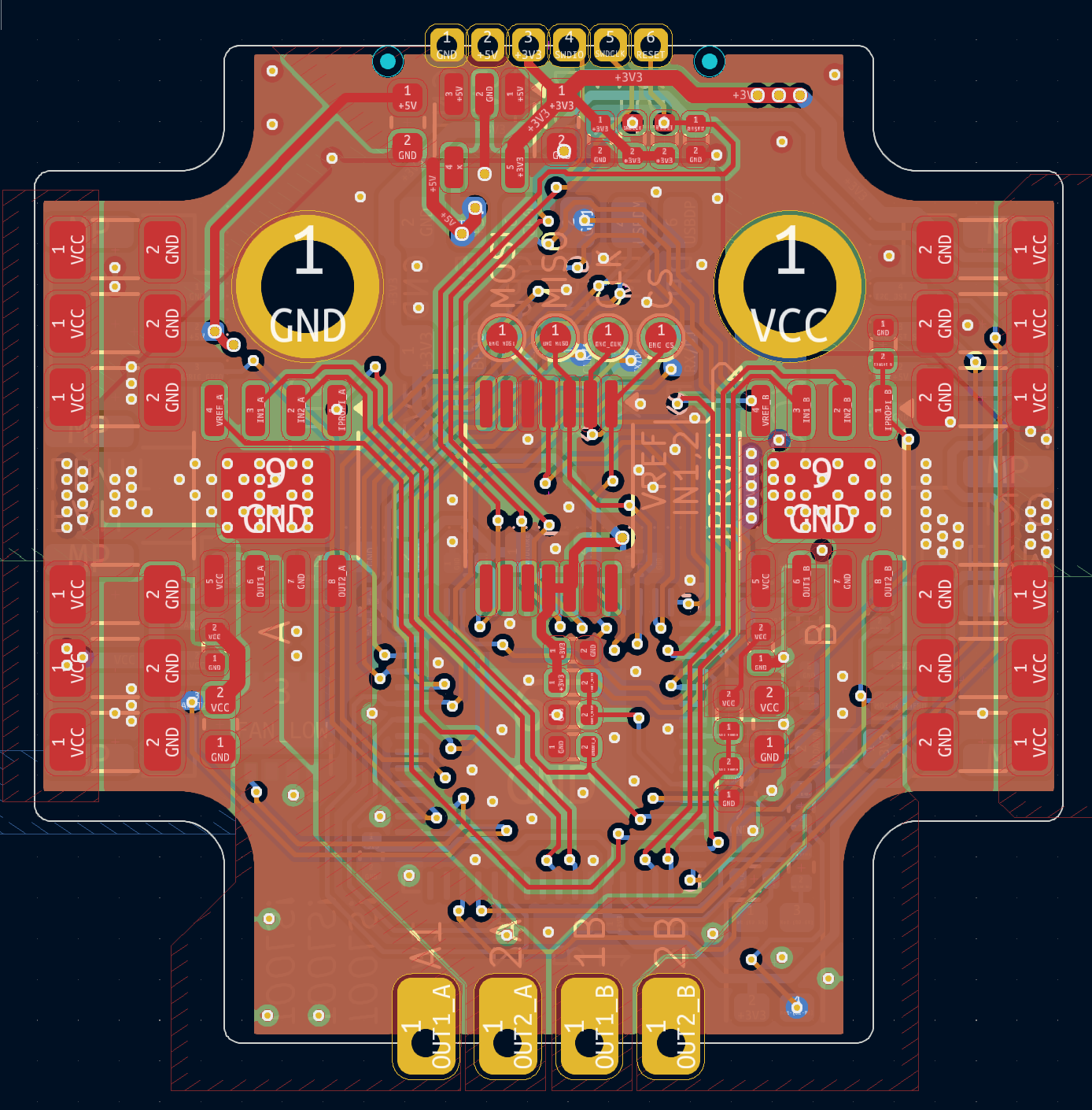
The layout. This one was tight, and it could probably use more bulk capacitance, but in the end it all fits OK. I did have to get a little fancy with the internal layers - only time will tell if I committed any GND plane sins.

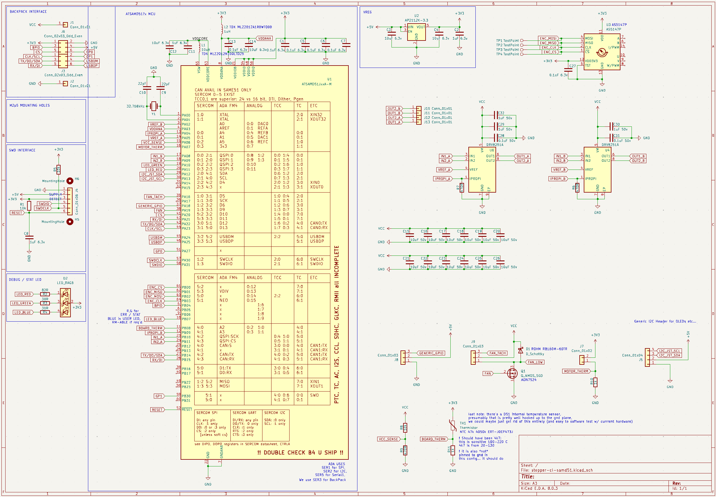
The schematic… thanks to the DRV8251A, and to the modular PHY, it’s pretty simple: encoder, 2x hbridge, voltage regulation for the MCU, thermistor, some plugs, and the fan driver… RGB LED as a treat. I’ll publish the harware properly someday, I promise.

I picked the DRV8251A because of it’s specs (50V, 4.1A, nice!) but mostly because of it’s feedback. The bridge contains a current mirror output on the IPROPI pin that outputs 1575uA/A of current flowing through the bridge. By sticking a resistor on that output (to make a voltage that is proportional to the output current), we can measure that on our microcontrollers’ ADC.

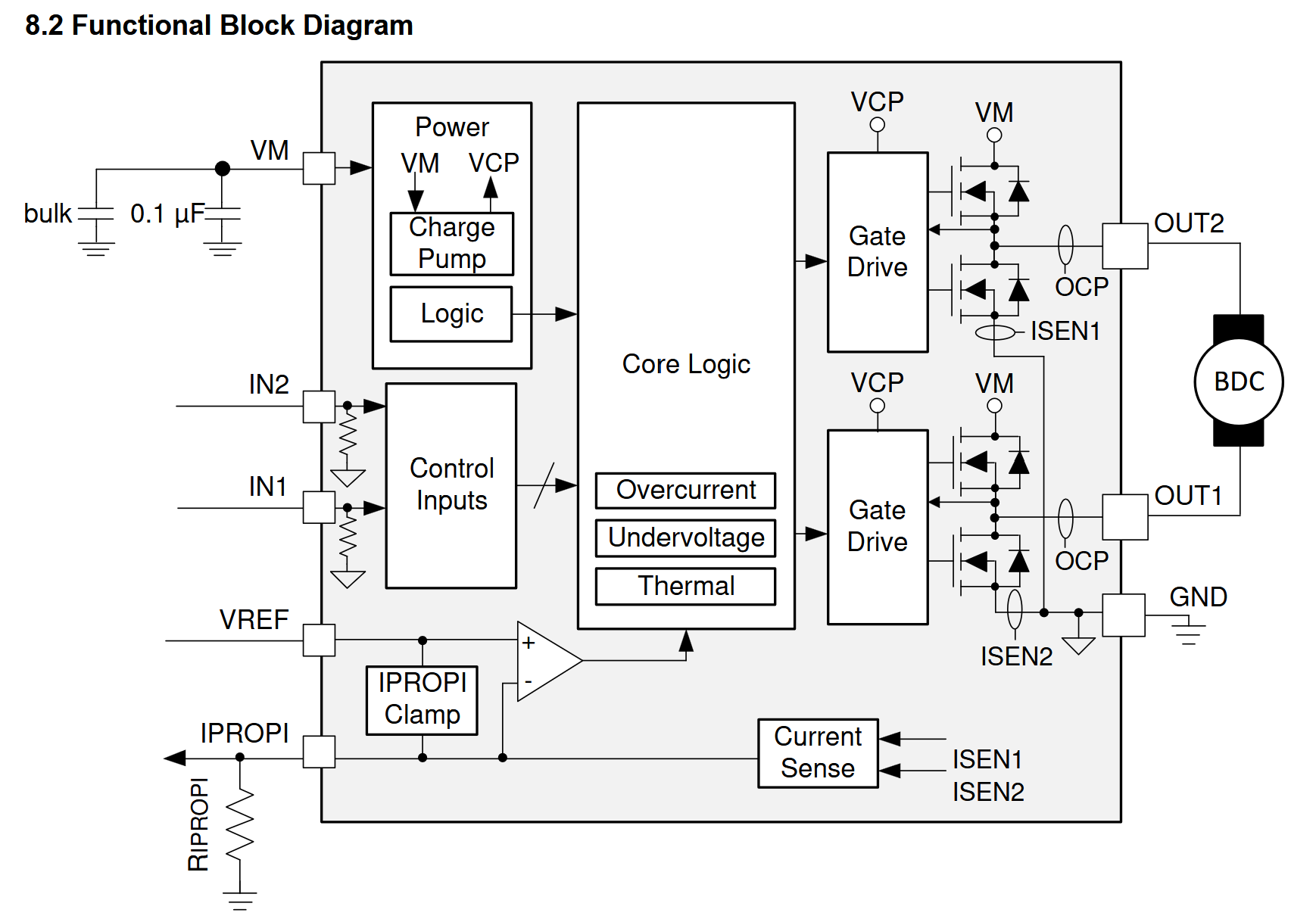
The DRV8251A block diagram. Mostly a standard hbridge, but including this current mirror, which we can use to measure current in the motor stator (and so, the magnetic field). Note that the one output pin IPROPI combines inputs from two measurement devices ISEN1 and ISEN2 … this will cause us to have to do some tricks later on.

The FOC Algorithm

The controller is really two main loops. Key inputs are encoder position and current readings (left top, bottom). We use encoder readings to correct for position disturbances (or hit target speeds / trajectories etc) (top loop). We also use it to commutate the motor (bottom).

FOC’s power is that it works well across a wide range of speeds, and uses the entirety of the motor effectively… it is smooth, torque-ey, and silent when implemented well. However, it requires that we have an accurate reading of the rotor’s position and readings of the current in the windings - both of which require additional hardware (as opposed to i.e. an open loop driver). FOC also requires that we tune a few different controllers: the PI controllers in the current loop, three gains in the rotor position observer (more on that later), and PIDs for position or speed loops that will get rolled on top of the core FOC driver. These are some of the things that we want to tune either automatically or with some information from a motor model.

The Magic: Current Control in a Stable Reference Frame

As mentioned, FOC works by placing target current on the quadrature axis of the rotor. We can’t directly control current in the stator, only voltage. This means that we need to sense current, and write a controller that dials voltage up and down in order to hit the right current. This would be enough to get started, but we would end up with rapidly changing current targets - as the motor spins, the target current vector rotates as well. This is where the magic of FOC is: it lets us do that current control in a reference frame that rotates alongside the rotor.

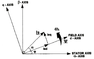
Via ResearchGate ‘Review on FOC of Induction Motor’ - the dq frame is aligned with the rotor: d axis current doesn’t do any work, but q axis current generates torque. Open loop steppers blindly rotate current in circles and take for granted that the rotor follows pretty closely, but lots of energy is wasted because only the misaligned current does work.

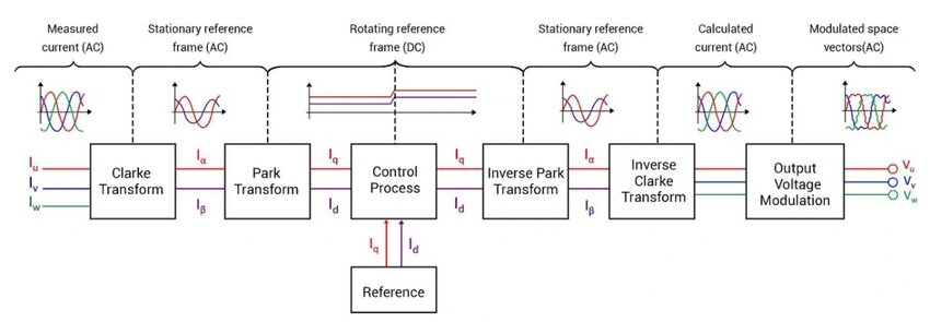
Via ‘FOC Implementation using STM32F103…’ (doi). This diagram depicts FOC for a three-phase BLDC, our two-phase stepper doesn’t require the Clarke transforms, just the Park transform and its inverse. FOC basically lets us control motor currents in a stable reference frame, i.e. the frame that moves alongside the motor’s rotor. Without these transforms, our current controller’s setpoint would be rapidly swinging around, making tracking much more difficult - and probably impossible at high speeds.

While I was working this out, I made a small test code in python to help make sense of the transforms before I wrote them into the firmware.

steps = np.linspace(0, 3 * 2 * np.pi, 1000)

x_in = np.cos(steps)
y_in = np.sin(steps)
# t_in = (np.arctan2(y_in, x_in) - np.pi * 0.6) % (2 * np.pi) - np.pi 
t_in = np.arctan2(y_in, x_in)

def xy2dq(theta, x, y):
    d = np.cos(theta) * x + np.sin(theta) * y 
    q = -np.sin(theta) * x + np.cos(theta) * y 
    return d, q

def dq2xy(theta, d, q):
    x = np.cos(theta) * d - np.sin(theta) * q 
    y = np.sin(theta) * d + np.cos(theta) * q 
    return x, y 

d, q = xy2dq(t_in, x_in, y_in)
x_out, y_out = dq2xy(t_in, d, q)

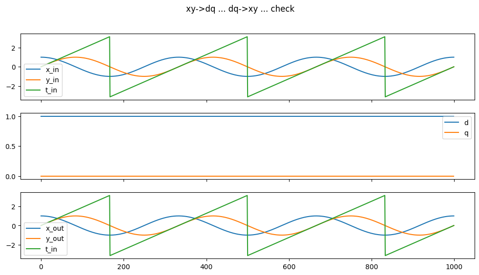
My transform test. At the top, two example ‘measurements’ ‘x_in, y_in’ and the reference angle ‘t_in’… these are transformed into the stationary dq frame (middle) and then back (bottom).

I called these transforms simply xy2dq and dq2xy, (or ab2dq …) but they are properly known as Park and Inverse Park. In FOC for a stepper, we don’t need the Clarke components since we already have two orthogonal basis vectors.

Current Sensing

I did the usual hardware setup to read the encoder and write some basic PWMs into the hbridges, and then got into measuring current. My ambition was to simply spin the thing around in open loop voltage mode and then look at currents coming back, to start to piece together the rest of the controller. In particular I was curious to see what the phase delay between voltage and current was, since I figured there was lots of motor physics to learn with that data.

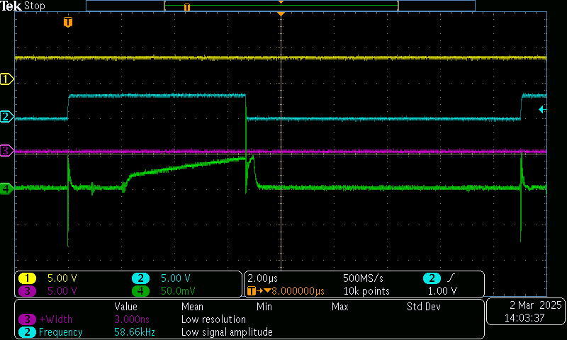
First trace I saw on the scope, CH1 (yellow) is an inactive debug pin, CH2 (blue) and CH3 (purple) are IN1 and IN2 on one of the hbridges, and CH4 (green) is IPROPI

This was encouraging: with previous hardware, current sense output was really noisy, and this is nice and clean. There’s a brief switching time (2us here) when I first switch the hbridge on (CH2 goes HI), then we see current rising in the winding, before it goes off again. But we see these nasty current spikes at startup and at the end of the pulse.

I hadn’t looked very carefully at the hbridge’s ‘truth table’ though, and at this point I was actually driving the thing into high-z state during the PWM off times. This would brake the motor excessively - it’s also known as fast-decay - it totally shuts the stage off, and causes the windings to generate lots of voltage… basically, we spun them up, and now there is a magnetic field in the windings that can’t just instantly turn off - so voltage rises as the energy tries to fight its way out of the winding. What we really want is to let the little current pulse that we created during the on state to keep looping around in the windings, it’s free real estate. This is kind of similar to using a flyback diode on a low-side switch: we give current in a winding a place to go during PWM off-times.

The hbridge ‘truth table’ - when we switch IN1 and IN2 to LO, we put the bridge in ‘fast decay’ mode - instead, we want the thing to always circulate current through the two low-side fets, and then turn one-or-the-other high-side fets on momentarily to generate more current.

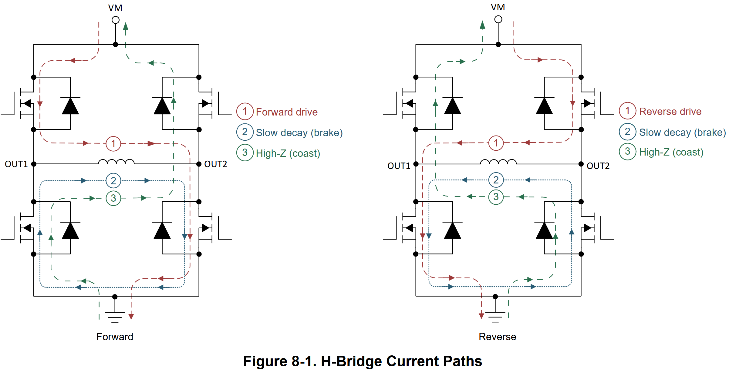
The hbridge current paths, corresponding to the IN1/IN2 states above.

So the real strategy here is to set both pins HI when the ‘voltage’ request is LO and then flip one side LO when the voltage request is issued in that side of the bridge’s direction - this little inversion is one of many small gotchas/headaches in this kind of firmware and basically requires that we write the PWM driver by hand. So it was into the datasheet for me.

In this firmware I’m using the SAMD51’s TCC module - Timer/Counter for Control which is a relative joy to use, but probably only because I am already familiar with the chip. Here I simply flipped the polarity of each output channel on IN1 and IN2 and then I operate them based on a signed pwm request value.

void apply_pwm_hbridge_a(int16_t duty){
  // no -ves into the TCC 
  uint16_t abs_duty = abs(duty);

  // flip dir. based on sign 
  uint16_t cc_in1, cc_in2 = 0;
  if(duty > 0){
    cc_in1 = abs_duty;
    cc_in2 = 0;
  } else {
    cc_in1 = 0;
    cc_in2 = abs_duty;
  }

  // write to hardware 
  TCC0->CCBUF[HBRIDGE_CC_CHAN_A_IN1].reg = cc_in1;
  TCC0->CCBUF[HBRIDGE_CC_CHAN_A_IN2].reg = cc_in2;
}

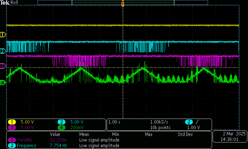
CH2 is PWM into IN1 and CH3 is PWM into IN2 - CH4 is the IPROPI pin at the ADC. I am driving a triangle wave -ve -> +ve, and we see positive current measurement in either direction. The small aberrations are me rotating the shaft by-hand - this changes inductance in the stator (and generates some BEMF voltage), so we can see the effects on the current trace.

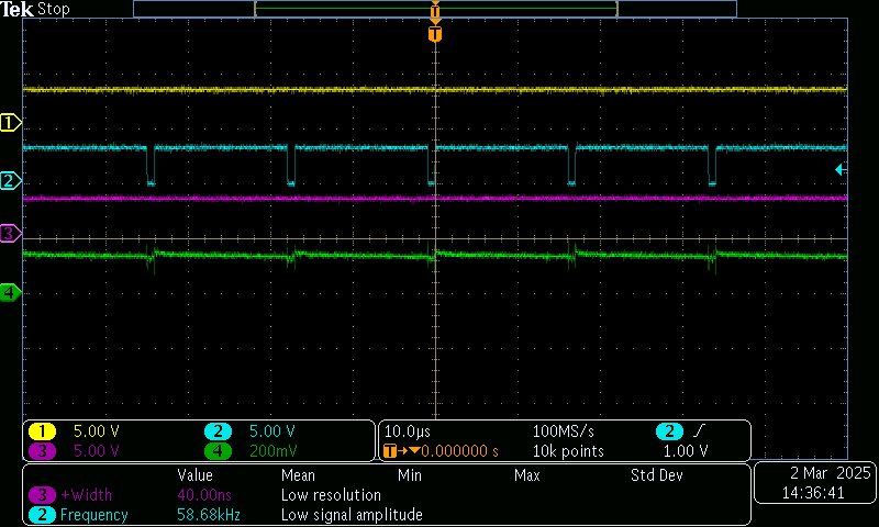
As above, but zoomed in. We can see the short ‘on’ pulse happens when IN1 goes LO - the current rises during this interval. Then, in the slow-decay state, the current gently decreases, before it is lifted again at the next pulse…

The plot above is what we want to see with a motor controller: the motor is ‘basically a big inductor’ that is filtering the pulsed voltage (blue) into a steady stream of current (green).

PWM Aligned ADC Sampling

Looking at the current on the scope is cool and all, but we want to read that into the microcontroller to do control with it. So here comes one of the tricks we can pull with a microcontroller that simply isn’t possible on more general computing devices: we configure the ADC so that it samples exactly when one of the TCC channels is triggered.

This SAMD51’s TCC has 8 channels in total, and I am using four already for the PWMs (they are configured as outputs). I can setup an additional channel to trigger one of the SAMD51’s event channels - these are like little hardware dataflow lines that we can use to communicate from one peripheral to another. That event channel is then connected to the ADC, where it triggers a sampling event.

This is a bit of a PITA to setup, but the timing is important. Firstly, it helps us to sample away from any noisy spikes on the line during the switch, and it lets us sample when we know what states the gates are in - this last part is more important.

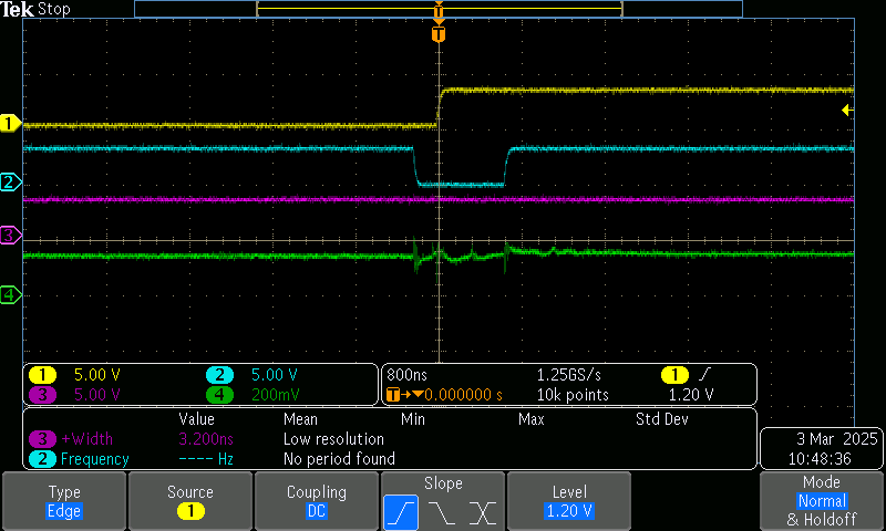
CH1 is a debug pin that I toggle in an interrupt activated by the event channel that triggers the ADC reading… so, it flips when the ADC is triggered. Here, I trigger it just after the IN1 gate goes LO.

I spent a while trying to get this right.

Originally I was triggering the ADC in the middle of either side of the PWM phase, i.e. halfway through the ‘off’ part of the cycle or halfway through the ‘on’ part of the cycle - I thought that due to the slow decay, I would always be measuring valid current and the precise timing was just useful to avoid noisy transitions.

The current reading is unsigned, as in we don’t know which way it is flowing through the hbridge when we sample the IPROPI pin if it’s in slow decay because the measurement is taken from whichever of ISEN1 or ISEN2 is largest… recall from the earlier block diagram of DRV8251A. I had figured that, looking at previous states from the system, it would be easy to reason about the direction of the current - but I soon realized that I needed a way to deterministically ascertain the sign of the reading…. the current loop is far too fast to be messing about with observers etc.

The real solution is somewhat counter-intuitive: during every pwm cycle, we need to flip the hbridge on in both directions for some amount of time. For example, if we are driving the bridge FWD at 20% duty over a 1040us period we drive:

• IN1=HI, IN2=LO (forward) for 220us, sampling the ADC (reading is FWD signed)
• IN1=HI, IN2=HI (coast) for 800us,
• IN1=LO, IN2=HI (reverse) for 20us, sampling the ADC (reading is REV signed)

Basically, we insert this minimum on-time for both directions, and sample the phase at the instant where we know the sign of the current measurement. This required that I re-write the PWM driver and the ADC sampling events.

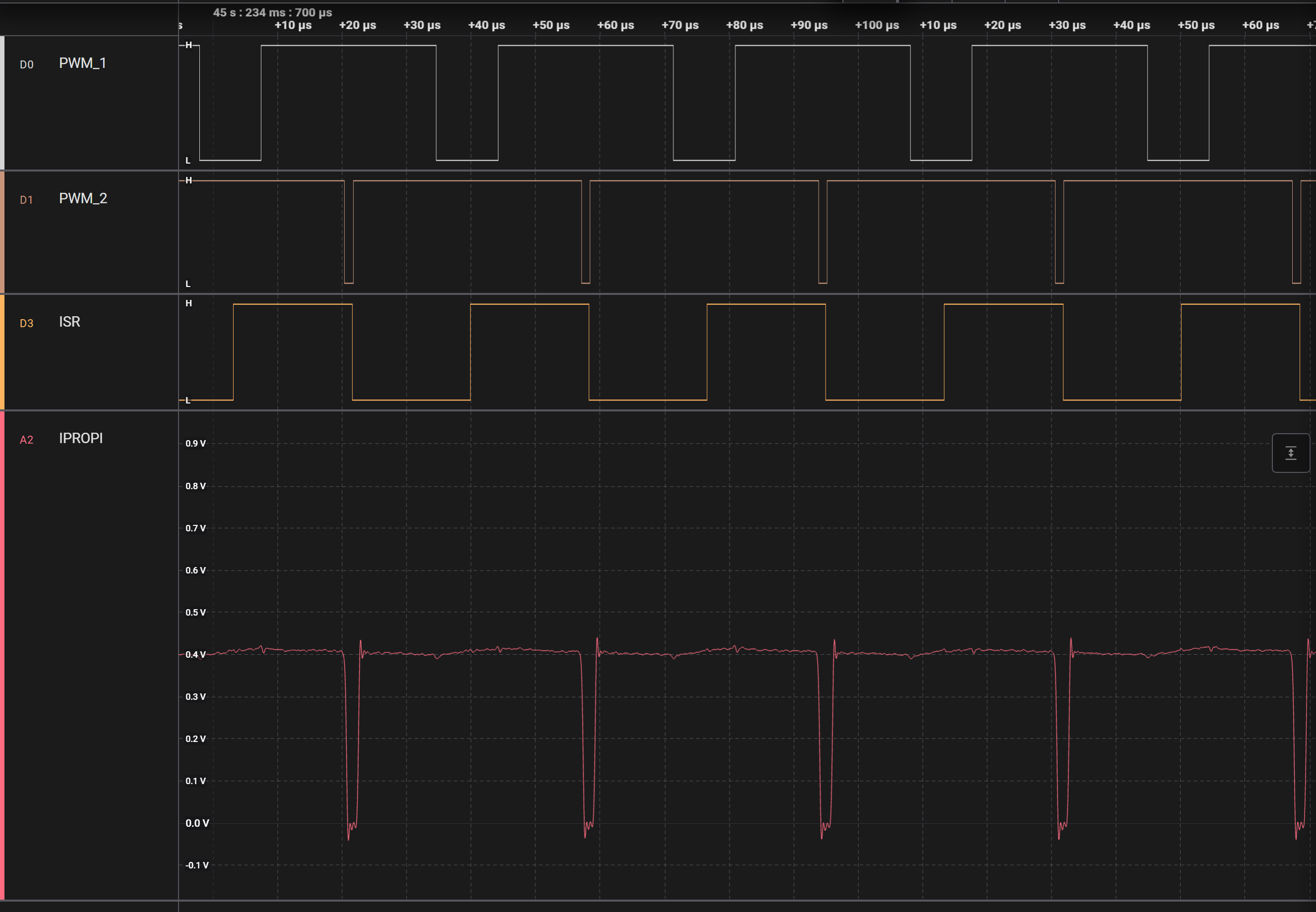
Traces from a Saleae logic analyzer, showing PWM to IN1 and IN2. The bridge here is driving in reverse: IN1 spends more time ‘down’ than IN2 does, driving current backwards through the bridge on average. We additionally pulse the bridge FWD for a short duration, during which cycle the IPROPI output (red) flips to show us how much current is flowing in that direction. The ADC is sampled during the middle of both pulses (sample timing is illustrated with the ISR line toggles).

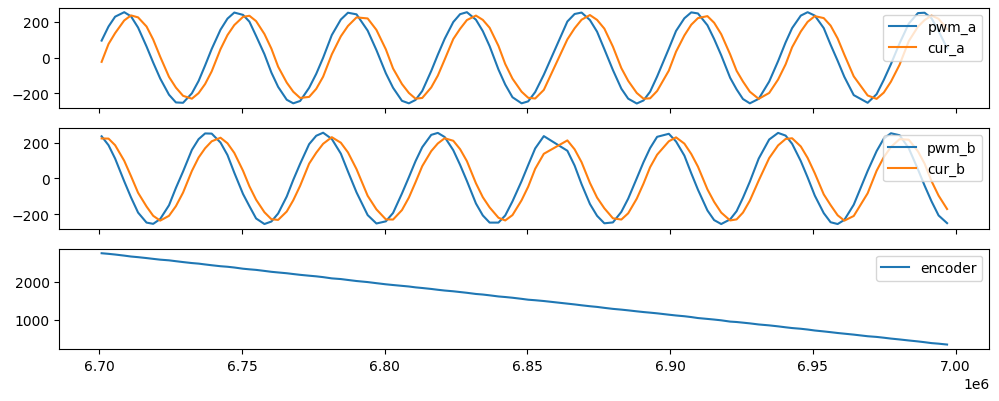
With two measurements, one in each direction, I could finally ascertain the signed current measurement from hardware, no fooling required. In these plots, you can see the phase delay between i.e. pwm_a and cur_a…

To set this up in hardware, I flipped the PWM’s WAVEGEN mode to use dual-slope pwm - this is a mode where the TCC counts up until TOP, and then back down to ZERO (figure below). I then flip the polarity of the second output channel, so that it goes LO around the TOP of the wave, and the first channel goes LO during the bottom of the wave (eliminating any overlap of the two LO signals, which would put the bridge into fast decay mode).

Then I have to trigger the ADC at both pulses. For this, I generate an event out of the TCC’s overflow (OVF) event, which (in this pwm mode DSBOTH) is fired at both the top and the bottom of the wave. That even triggers the ADC sample, and then an ISR picks up the readings and stashes them (and reads the TCC’s COUNT register to ascertain which side has just been sampled) - they’re consumed in a subsequent ISR that runs the current loop.

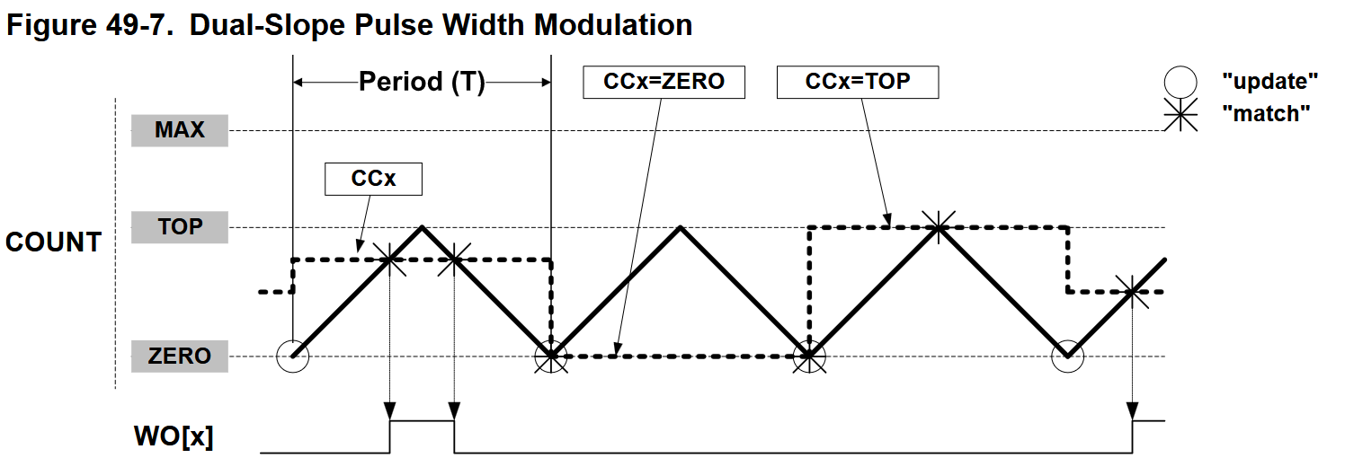
The SAMD51’s Dual Slope PWM mode, (datasheet: 49.6.2.5.6). I inverted pins such that IN1 to go LO at TOP and IN2 goes LO at ZERO - this eliminates a fast-decay state that would occur during the small overlap that would occur if I used ‘normal’ PWM. I also use the TOP and ZERO overflow events to trigger ADC readings at those specific moments.

I tried to set this up with the minimal number of ISRs, since switching contexts is costly. Both ADC0 and ADC1 are both setup on the D51, with ADC0 sampling one hbridge and ADC1 sampling the other. Since I am using one TCC to control both sides of the motor (via four output channels to two hbridges… two channels each), the samples (and ISRs) are aligned across hbridges, meaning I can use one ISR to collect both samples.

Interleaving Other ADC Readings

For one last gotcha, I had to get the other ADC readings to happen in the middle of all of these events. Most microcontrollers only have a few real ADCs, that are ‘muxed’ onto many different input channels. For example in an arduino with nine ‘analog in’ pins, the MCU might only have one actual ADC. When we tell arduino to sample on (1) and then on (2), it actually reconfigures the ADC when we call the function, then triggers a sample and waits for it to complete. This all takes up valuable time, since the conversions don’t happen in one clock cycle (it can be 50 or more clock counts).

To avoid these hangups, I added a modal switch that swaps the ADC channels to my three other analog inputs on the board (on-board thermistor, off-board thermistor and a voltage divider on VCC). Right now this happens only two or three times a second, which is plenty fast for those readings. I should improve this later, as it briefly disables the current readings during those intervals (the controller just uses the previous measurement…). To do better, I can sneak a third sample in without interrupting the main current sampling instants.

The thermal information is slow, but the VCC might be interesting to watch at higher frequencies - doing so could be a good indicator that more bypass capacitance needs to be added, for example, and precise input voltage is important to measure if we are going to dynamically fit motor models.

Calibrating the Encoder

OK: we have current readings, so we can roll a current controller to point the magnetic field in whichever direction we choose. However! We need that pesky reference angle \(\theta\).

This is why we have the encoder: it reads [0, 16383] (14 bits) and it’s absolute, so the readings are indexed in the same manner when we restart the controller. However, we need to know how mechanical angles correlate to electrical angles. Recall that we have 50 full electrical rotations for every mechanical rotation, and we have some offset. The full 14 bits are useful here, since it means we have ~ 328 counts per electrical phase. Some other common encoders for BLDC FOC have only 11 or 12 bits of resolution, i.e. 41 or 82 counts per electrical phase.

To gather data for this, I spin the motor around in open loop voltage mode - I sweep forwards and reverse at a few different speeds, and ingest time stamped readings of the speed, voltages, current, and encoder readings. Using that raw data, I can turn A, B voltage and current readings into phase angles, and then plot them against the encoder angle, that’s below.

The electrical phase of the current is the best estimate of the rotor’s actual position during these samples, since that’s where the magnetic field is pointing, and we are assuming that the rotor is tracking that. However, it’s easy to spin the field too quickly and loose rotor tracking, so the calibration routine needs to discriminate stalled rotors and eliminate those data points. It’s also important that we use an equal number of samples from each speed and direction, since the rotor actually lags the current vector by some amount - more when the thing is moving faster.

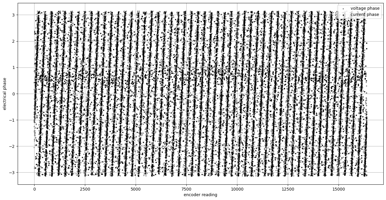
Encoder readings potted on x, with voltage and current phases (grey, black) plotted on y. We want to fit a function that returns the rotor’s electrical phase for any given encoder reading.

This is a sensible way to look at the data, since it’s basically the function we want to fit: for any encoder reading, return the electrical angle. But fitting it in this modulo’d space is insane, although I will admit that I tried to do so for a minute. Quentin ended up helping me out, and showed me np.unwrap(...) which unrolls both sets of periodic data, where they look like more normal functions. For convenience, we also do the fit in [-pi,pi] on both axes (i.e. normalizing the encoder readings). Then we can fit them with a little scipy.optimize.minimize …

# returns electrical phase, given encoder phase 
def fit_func_linear(params, enc_phase):
    return enc_phase * params[0] + params[1]

def loss_linear(params, enc_phase, tru_cur):
    fit = fit_func_linear(params, enc_phase)
    err = fit - tru_cur 
    return np.sum(np.square(err))

x0 = np.array([50, 0])

res = scipy.optimize.minimize(loss_linear, x0, args=(encs, curs), tol=1e-12)
xf_lin = res.x 

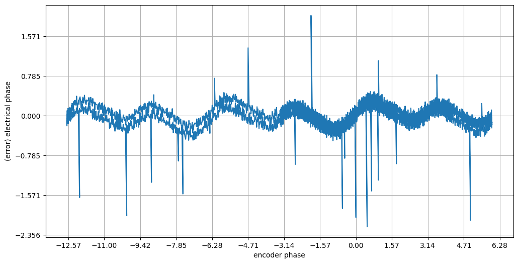
Errors after a linear fit - looks a lot like CORDIC error.

The linear fit is pretty good, but has this odd looking error… there’s a sinusoid in here at twice the frequency of the encoder phase, and one at the frequency. As it turns out, this is probably mostly error from the AS5047’s CORDIC unit, which is an old computational / hardware library that approximates the atan2 function - something I learned as we investigated this error.

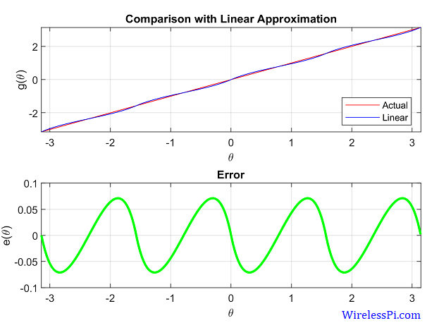
Via wirelesspi.com - Coordinate Rotational Digital Computer (CORDiC) is a set of lightweight trigonometry approximations for embedded devices and ICs. The atan2 function is particularely common / useful for translating between cartesian and polar coordinates… but it has this error, which looks about identical to the error term that drops out of a linear fit from our encoder.

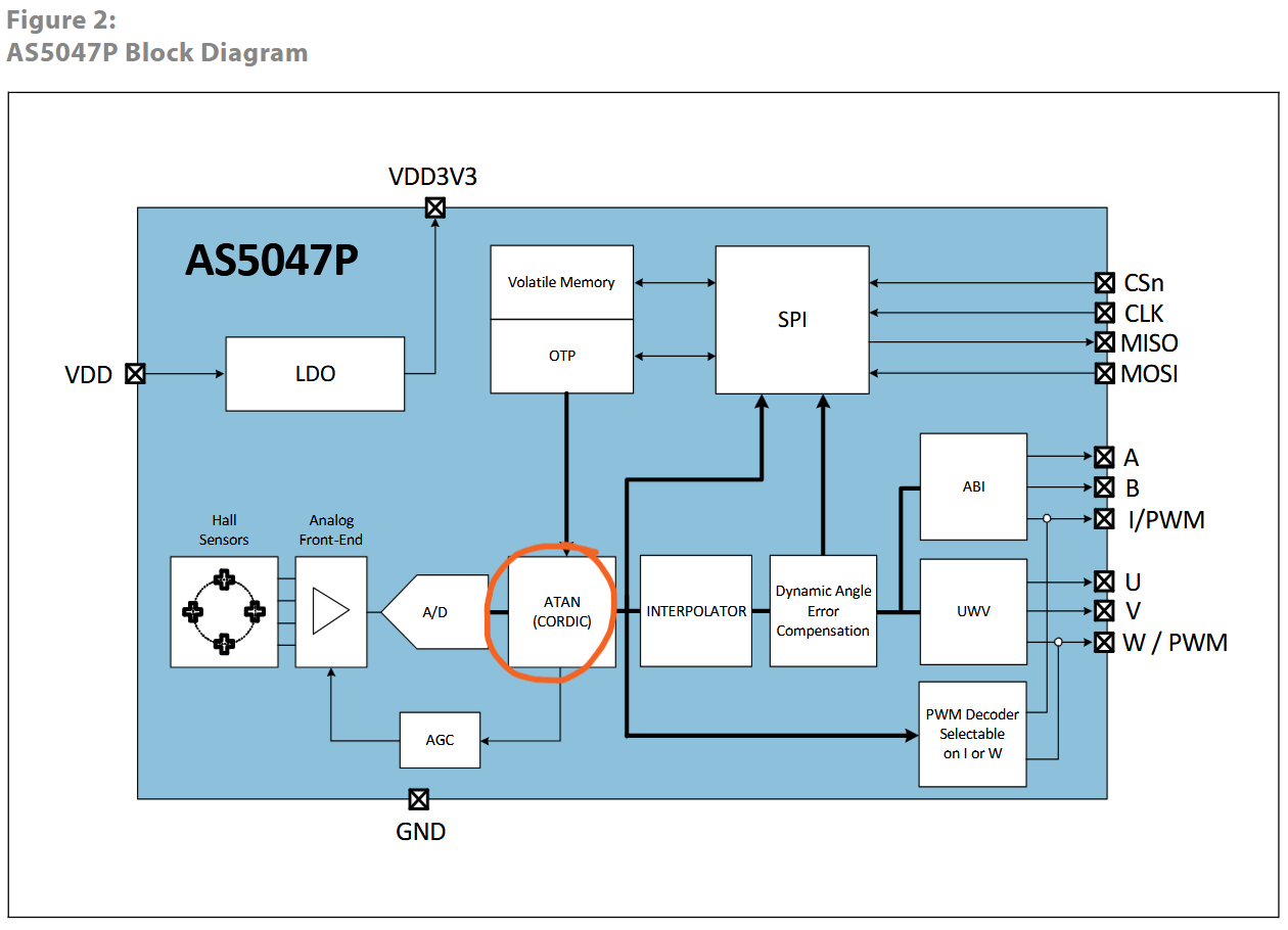
Block diagram for the AS5047 encoder, showing the ATAN CORDIC block, which is what the encoder uses to translate A, B magnitudes from its hall sensors to an angular reading.

Probably the best way to do this would be to draw up the actual CORDIC error pattern as a function and then fit parameters for offset and scale of that to this data, but instead we just stuck two more sinusoids in to fit: one at 2x the encoder frequency and one at 1x. This worked great, or at least well enough for now.

# returns electrical phase, given encoder phase 
def fit_func(params, enc_phase):
    lin_fit = fit_func_linear(xf_lin, enc_phase)
    major_period = params[0] * np.sin(2 * enc_phase + params[1]) + params[2] 
    minor_period = params[3] * np.sin(enc_phase + params[4])
    return lin_fit + major_period + minor_period

def loss(params, enc_phase, tru_cur):
    fit = fit_func(params, enc_phase)
    err = fit - tru_cur 
    return np.sum(np.square(err))

x0 = np.array([1, 0, 0, 1, 0])

res = scipy.optimize.minimize(loss, x0, args=(encs, curs), tol=1e-12)
xf = res.x 
final_loss = loss(xf, encs, curs)

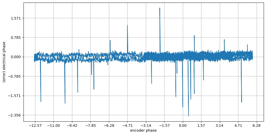
Including two more sinusoids into the fit (one at 2x encoder frequency, and one at 1x), we get rid of most of the rest of the errors. Those noisy little spikes are a bona-fide source of noise in the system: the SPI transaction with the encoder seems to occasionally suffer from one-flipped-bit… I haven’t tracked that down yet.

Now that we have our fit, we can stick it back in hardware. For now what I’ve done is just had numpy pretty-print a table into the console that I copy and paste into a lookup table (LUT) style thing. I do the modulo arithmetic in python as well - and re-scale everything to the units that I’ll be using in the embedded system.

// in lut_encoder.h 
const int16_t LUT_ENCODER_2_ROTOR_ELECTRICAL_PHASE[16384] = { 
  //...
  //...
};

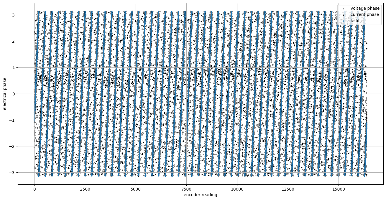
Periodic data as-above, now with 'le fit'

LUT Trigonometry for the Transforms

Speaking of units and data types, we now have to do a bunch of arithmetic in embedded, and so we are going to add even more lookup tables. If you recall the controller outline above, you’ll notice that i.e. native data types for encoder and motor phase are [0-16383] …

Note elec. phase LUTs are [0-16383].

Well! That’s because we are doing trigonometry in here with more LUTS. This is a pretty common trick so I won’t go into too much detail, I did find a neat new LUT generator here to use…

For those unfamiliar, the gist is simple: we take some function \(f(x)\) and then discretize it across some integer range… in this case mapping \(x \in [0, 2\pi] = [0, 16383]\) and then we calculate all of the possible results ahead of time and simply write them into memory, in a lookup table. Using i.e. const ... will tell the compiler to write that into Flash (not RAM), saving some valuable space. Then to evaluate, we simply say \(f(x) =\) LUT[x].

It is particularely useful with periodic functions aka sin/cos, where the input can wrap (i.e. \([0,2\pi] == [2\pi,4\pi]\)) to set the span of the input at some power of two: i.e. in this case the input is 14 bits. This means that we can use a bit mask to replace the modulo operator we might otherwise need…

/** Generated using Dr LUT - Free Lookup Table Generator
  * https://github.com/ppelikan/drlut
  **/
// Formula: sin(2*pi*t/T) 
const float_t LUT_TRIG_SIN_LUT[16384] = {
  ///
  ///
};

// ingests theta = [0 -> 16383] == [0 -> 2PI] 
// returns float [-1.0 -> 1.0]
float lut_trig_sin(int16_t theta);

// ingests theta = [0 -> 16383] == [0 -> 2PI] 
// returns float [-1.0 -> 1.0]
float lut_trig_cos(int16_t theta);

typedef struct{
  float d;
  float q;
} lt_dq_t;

typedef struct {
  float x;
  float y;
} lt_xy_t; 

lt_dq_t lut_trig_xy_2_dq(int16_t theta, lt_xy_t xy);

lt_xy_t lut_trig_dq_2_xy(int16_t theta, lt_dq_t dq);

// we can wrap 14 bits using a mask, meanig we do periodic maths 
// implicitly / bitwise - fast ! 
#define LUT_TRIG_THETA_WRAP_MASK 0b0011111111111111

float lut_trig_sin(int16_t theta){
  // wrap for 0-16k 
  theta = theta & LUT_TRIG_THETA_WRAP_MASK; 
  return LUT_TRIG_SIN_LUT[theta];
}

float lut_trig_cos(int16_t theta){
  // same wrap, shift phase by 90' 
  theta = (theta + LUT_TRIG_HALF_PI) & LUT_TRIG_THETA_WRAP_MASK;
  return LUT_TRIG_SIN_LUT[theta];
}

Then the transforms themselves are pretty simple - using a custom struct for dq, xy frames - and (since the SAMD51 has an FPU) I do most of the rest of the maths using floats - nice and simple.

lt_dq_t lut_trig_xy_2_dq(int16_t theta, lt_xy_t xy){
  lt_dq_t dq;
  dq.d = lut_trig_cos(theta) * xy.x + lut_trig_sin(theta) * xy.y;
  dq.q = -lut_trig_sin(theta) * xy.x + lut_trig_cos(theta) * xy.y; 
  return dq;
}

lt_xy_t lut_trig_dq_2_xy(int16_t theta, lt_dq_t dq){
  lt_xy_t xy;
  xy.x = lut_trig_cos(theta) * dq.d - lut_trig_sin(theta) * dq.q;
  xy.y = lut_trig_sin(theta) * dq.d + lut_trig_cos(theta) * dq.q;
  return xy;
}

Filtering Encoder Readings

By now all of the nuts and bolts are together, but the larger challenge of controlling the motor well is still with us. One of the things that has caused trouble for me in the past is de-noising the position reading from the encoder, and also estimating the thing’s velocity (and acceleration, if possible) using that data.

Position is obviously useful for closing position loops, but velocity and acceleration are great to have. For example in FOC, we can use the velocity to predict the rotor’s position in between encoder samples - so i.e. if we are sampling our encoder around 10kHz but we want to run our current controller at 30kHz, we need two extra predictions. We might also want to replace the position PID with a proper LQR controller, and velocity measurement there would be critical… The PID controller is also making a continuous estimate of the position error derivative which is ~ at least highly related to velocity, so we might be able to filter once and use the information twice - etc, you get the picture, it’s useful to know how fast you’re going haha.

Taking discrete derivatives of position in order to calculate velocity is famously difficult to do without making really noisy signals, since we typically sample at high frequency and most of the change between measurements sample-to-sample is due to noise, unless we are going very quickly. We basically need to do some kind of averaging or filtering to get a sensible output, even with pretty good encoders.

Kalman4Idiots

I was originally trying to crack this by writing a Kalman filter and, while I could get ChatGPT to spit out a good implementation of one, I still don’t entirely understand what it is doing. This is a real kind of moment where I wish I had eaten more of my maths vegetables in the past.

I then wrote this weird filter that turned out to have really good performance - it keeps a velocity estimate and uses that to improve position estimates (taking i.e. 20% of the estimate and 80% of the reading, depending on a setting), and conversely uses the position estimate as a basis for the velocity estimate (which is filtered using a normie exponential filter).

class Kalman4Idiots:
    def __init__(self, dt, alpha_pos, alpha_vel):
        self.dt = dt 
        self.alpha_pos = alpha_pos 
        self.alpha_vel = alpha_vel

        self.vel_est = 0.0 
        self.pos_est = 0.0 

    def update(self, measurement):
        vel = (measurement - self.pos_est) * (1 / self.dt)
        self.vel_est = vel * self.alpha_vel + self.vel_est * (1 - self.alpha_vel)
        
        pos_predict = self.pos_est + self.vel_est * self.dt
        self.pos_est = measurement * self.alpha_pos + pos_predict * (1 - self.alpha_pos)

        return self.pos_est, self.vel_est 

This actually worked really well, in fact I could tune it to about the same performance as the Kalman implementation (with the bonus that I had an intuition for the knobs I was dialling). These plots are coming from tests using data that I generated in numpy with some artificial noise - so I’m not actually sure how well this would work on real data.

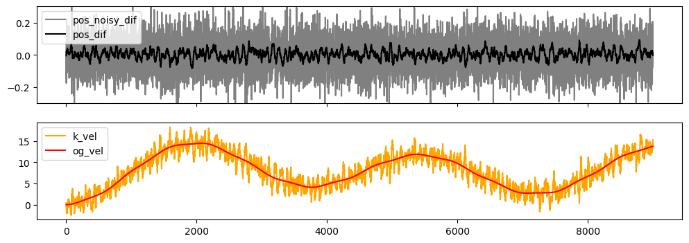
Performance of the Kalman4Idiots filter was surprisingly good.

A neat trick that I will probably stash for later - and that could presumably be extended into acceleration… but it works like shit when we have substantial changes to acceleration - unsurprising since it doesn’t have internal prior that acceleration might happen.

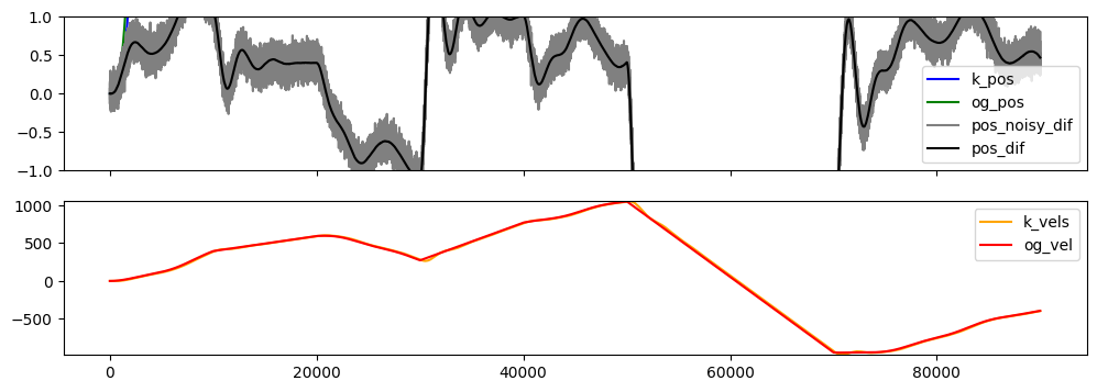
The same filter, but subjected to big changes in acceleration. The position estimate basically lags the real position by some amount that is proportional to the acceleration.

“Alpha Beta Gamma” Observers

I wound up learning (again) about observers - I originally saw these when I took Jacob White’s beginner controls class (IIRC it was 6.302)… I probably should have finished this project right after that class, but at least the seed was planted!

The basic idea is that we have a model of our system and we track its internal states. This one in particular is simple: we have pos, vel, accel, and the model just says that acceleration turns into velocity and velocity turns into position. At each time step we make a prediction, and we compare our prediction to the measurement. The difference is called innovation (unpredicted change!), and we can update our estimates using some amount of that innovation - i.e. three filter values (the alpha, beta and gamma) that are ~ related to our trust in the measurement.

class AlphaBetaGamma4Idiots:
    # alpha = position gain, beta = velocity gain, gamma = acceleration gain 
    # we assume position is slow to change (small gain), 
    # velocity is faster (larger), 
    # accel is nearly instant (arbitrarily big) 
    def __init__(self, dt, alpha, beta, gamma, vel_max, acc_max):
        self.dt = dt 
        self.alpha = alpha 
        self.beta = beta 
        self.gamma = gamma 

        # very-useful abs. bounds:
        self.vel_max = vel_max 
        self.acc_max = acc_max 

        self.pos_est = 0.0 
        self.vel_est = 0.0 
        self.acc_est = 0.0 

    def update(self, measurement):
        pos_pred = self.pos_est + self.vel_est * self.dt + 0.5 * self.acc_est * self.dt * self.dt 
        vel_pred = self.vel_est + self.acc_est * self.dt 
        acc_pred = self.acc_est # ... all change in accel is due to new info 

        # unpredicted change... 
        innovation = measurement - pos_pred 

        self.pos_est = pos_pred + self.alpha * innovation 

        self.vel_est = vel_pred + (self.beta * innovation) / self.dt 
        self.vel_est = max(-self.vel_max, min(self.vel_est, self.vel_max))

        self.acc_est = acc_pred + (self.gamma * innovation) / (0.5 * self.dt * self.dt) 
        self.acc_est = max(-self.acc_max, min(self.acc_est, self.acc_max))

        return self.pos_est, self.vel_est, self.acc_est 

I had a really hard time getting this to be stable until I added the vel_max and acc_max values… which are pretty easy to guess using system knowledge (and they don’t have to be too close to reality, just guesses with lots of overhead). Without them, what can happen is this:

• we make a measurement that causes us to make a big acceleration and velocity innovation
• the next cycle, our prediction is well ahead of the measurement, and now we dial it back in the other direction (overcorrecting)
• etc, until we hit np.inf

This one I was ablt ot tune up pretty well to my test data, and the addition of an internal acceleration state (while noisy…) is cool.

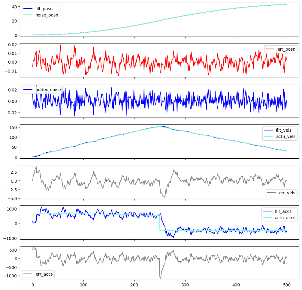
Output from this alpha-beta-gamma filter, showing good tracking for position and velocity, with noisy (but available!) tracking of an acceleration state.

I went ahead and implemented this in cpp on the device, so now I have states available in hardware, although I haven’t properly tuned it, which is kind of future work at this point. That said, the gains should be about the same from motor-to-motor, since they are only related to the noise that comes from the encoder, and that shouldn’t change drastically. Tuning the vel_max and acc_max is similarely simple: we should basically cap them such that they don’t allow the system to explode, which can be calculated easily if we know the time step taken between measurement / update steps.

Current Controller PI Gains

To get to the next steps, we need to tune the current controller gains. I learned that this is possible if we know the motor’s coil resistance \(R\) and inductance \(L\) - both of which are on the datasheet for this motor, and can be measured using this hardware, although I haven’t implemented that step yet.

\(k_p\) is the simplest, check it out: \(k_p = R\) - seems too good to be true, but consider the units \(V / A\) - i.e. how many volts should we apply to get one amp of current correction? That’s just ohm’s law.

\(k_d\) doesn’t exist, basically beacause there’s no / negligible inertia in the system, thank god.

\(k_i (V/A \cdot s)\) is messier - we want to pick a bandwidth for the controller first. We can use the electrical time constant to understand what a maximum bandwidth might be:

The time-constant is how long it takes for the system to hit ~ 63% of its final state, after a step input, so \(\frac{1}{\tau} = f_c = 680Hz\) represents the frequency that we can expect to swing the thing around. So, an upper bound on how fast our current controller can expect to operate. What still confuses me here is that this somehow applies in the rotating frame even though the underlying hardware is rotating much faster. As will appear later, my non-understanding of frequency-dependent impedance of the motor-as-and-inductor is causing some problems.

In any case we can pick this as a target bandwidth, and use \(k_i = 2\pi f_c \cdot L = 6.8\) (!)

I will say, I don’t completely understand this step, but it works terribly well so I am leaving the comprehension for next time.

A Position PID Loop, and Loop Timings

Once the core FOC layer and observer was working, this step was pretty uncomplicated: position estimate comes from the observer and the PID controller decides how much torque to put on the q axis of the FOC controller.

Tuning the gains is another question: it is easy to make the thing work, but difficult to make it work well. I get the sense that tuning in-general (of the current controller PI gains, of the observer gains, etc) is the main challenge for closed-loop motion systems, and (besides cost, which is actually not that great) is probably why most simple systems use open loop motors, or ‘closed loop’ motors that only use their encoders to recover lost steps.

Here I’m periodically updating a position PID’s setpoint, and plotting torque that the motor is using to hit that target. The gains aren’t execellent, and the inertia is huge relative the actuator, but it at least closes the loop across the whole system.

I also tightened up my loop timings at this point. The current controller bandwidth is way higher than I think is probably necessary, but it is pretty cheap to run. The spline interp / position control is fast enough, but ideally we would actually poll the encoder at extremely high speed, since commutating the many-pole-pairs of the stepper motor requires really high frequency position information… in fact, in a couple of cases I saw current sinusoids on the oscilloscope that were only two or three PWM periods long - meaning the motor rotated through one-half electrical rotations in as much time.

• 30kHz PWM
• 30kHz Current Control
• 15kHz Spline Interpolation
• 15kHz Position Control

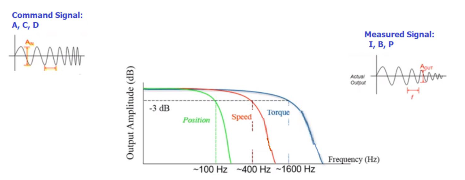
Via app note 103 / 102 from Oracle Robotics. Shows ‘typical’ loop speeds for closed loop servo control - although this is likely to vary application to application and across motor sizes, with smaller inertias requiring more responsive control. These intervals are substantially larger than those that I implemented, probably typical of larger motors with less pole pairs, but also means that I could probably get away with less Hz if I could tune these loops like the experts.

To give myself some more overhead for all of this, I am running the SAMD51 at 180MHz - a little more than the ‘spec’ 120MHz. Using Platformio and Adafruit’s M4 Feather Core, this was a really easy config change. Internet suggests it can run at 200MHz, but I think I have it in a somewhat noisy environment so I will leave it here.

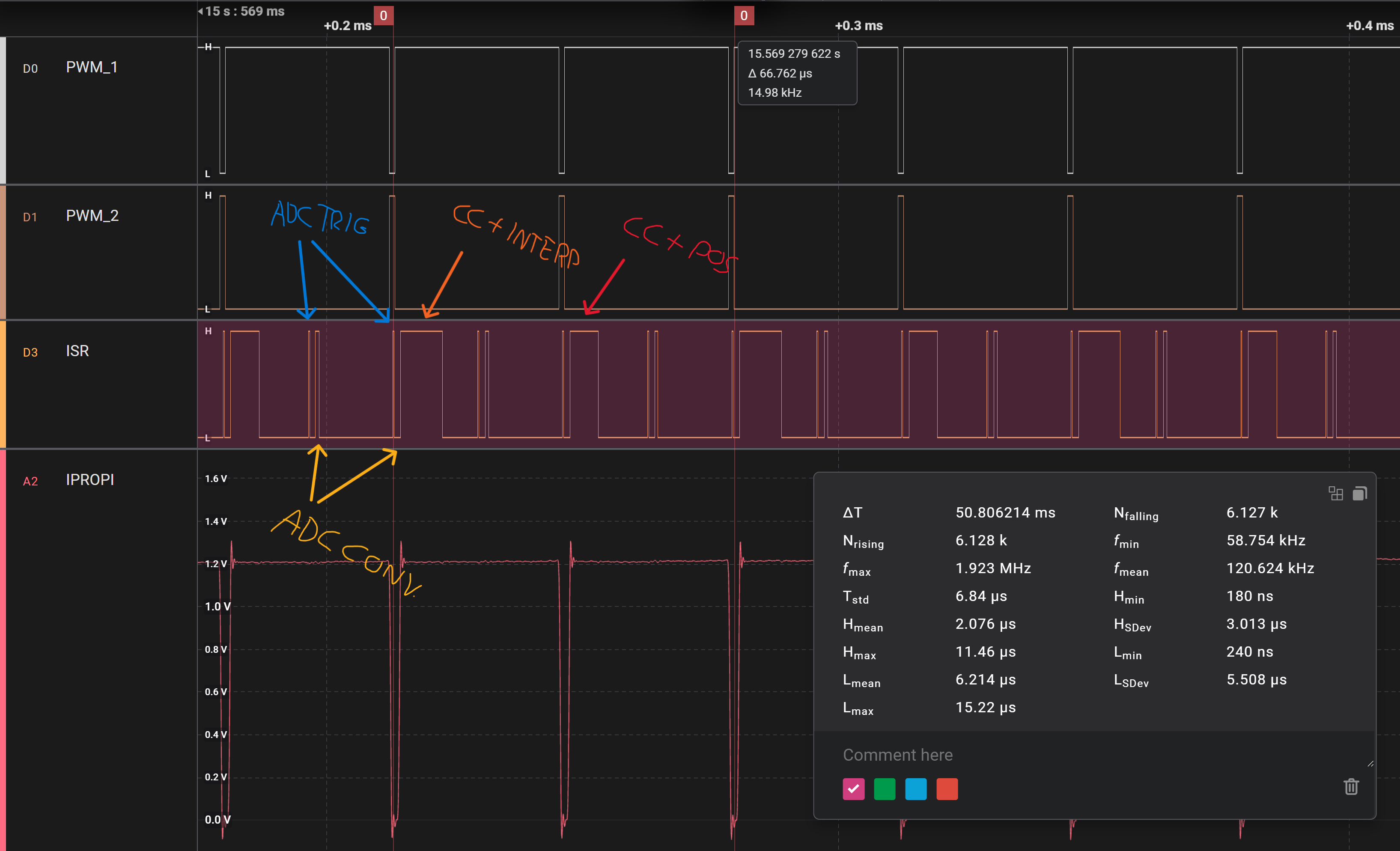
I have two ISRs here, and interleave operations. Basically the whole controller runs in these ISRs besides the interface, and it takes about 25% of the processor’s time to do so. Not pictured are the ISRs that handle the SPI transactions for the encoder. Each sequence is triggered by the TCC’s overflow or underflow, which sends an event to the ADCs to start a sample. That event also triggers the first ISR (the tiny slice), which records pin states during the sample time. The second ISR is the ADC’s conversion-complete signal, where we wake up again and pick up the new data. Then we either (1) go back to sleep if we are still waiting for the second ADC sample, (2) run the current controller, the interpolator, and tell the encoder to start acquiring a sample, or (3) run the current controller and position controller, using the new encoder reading. The interpolation step is the longest (up to 10us) since it is evaluating a basis spline and potentially incrementing through a buffer of control points.

Measuring Motor Parameters, and some Modelling

OK, with hardware it normally takes a long time to sort out the nuts and bolts, but then we get to do the fun stuff. That is the point we are finally at here; we get to (try to) learn some parameters for the motor-under-test (MUT)’s model, so that we can report torques while it is in use… so that we can model our machine systems / motion systems while we operate them! Modeling / understanding motor parameters also helps us to tune some of those nasty gains without thinking too hard.

Robots measuring their own forces is sometimes called proprioception, a term borrowed from biology for ‘the sense of self-movement, force and position.’ - i.e. the sense you use when you’re reaching inside the cheeze-its box to find that last morsel is proprioception.

In the case of most electric motors, output torque is more or less directly proportional to the current that is active on the q-axis, but we need to fit a few parameters in order to know how this current relates to torque.

I want to add a caveat here that this is something I am still learning about - so … don’t trust my maths, basically.

The Canonical Motor Model

It’s beautiful, but lossy.

• \(V_a\) is the voltage applied to the motor, i.e. v_a = vcc_supply * pwm_duty
• \(\dot{\Theta}, \ddot{\Theta}\) velocity and acceleration (rads)
• \(Q = torque = \ddot{\Theta}J\) is the identity for torque (Nm)
• \(R\) is coil resistance (Ohms)
• \(J\) is inertia of the rotor and whatever else is attached (kg \ m^2)
• \(k_d\) is damping due to friction (force / speed)
• \(k_e, k_t\) are emf and torque constants
• \(L\) is motor inductance

This model is what you’ll find if you’re studying DC motors, i.e. the brushed kind. With FOC, we do all of this work to commutate the motor… so that we can ignore that part when we make these models. To disambiguate, in these models the \(V, I\) terms are basically assumed to lie on the quadrature axis.

Once we fit each of these, we should be able to use \(k_tI\) to measure output torque - since we can measure current directly. Eventually I want to measure each of these automatically, but for now my process to find the physical constants was thsi:

• Measure \(R\) with a multimeter (it’s easy)
• Measure \(J\) by drawing the motor rotor in CAD, and having that software calculate it
• Measure \(L\) by reading the motor datasheet

A real measurement of \(L\) is probably the most important thing to improve the readings’ precision, same with actual \(R\) measurements, since the datasheet sepcs are for \(\frac{+}{-} 20\%\) (!). Even \(R\) changes by about 10 percent coil-to-coil in the same motor.

I also found that adding some real inertia to the motor is basically required, since the rotor’s own inertia is normally so small as to be negligible in the face of the torque it can produce. That is, when we spin up just the rotor, the change in direction is so fast that we can’t really sample any of the dynamic states that happen during that turnaround. So: enter big disk of PLA, the world’s simplest dynamometer.

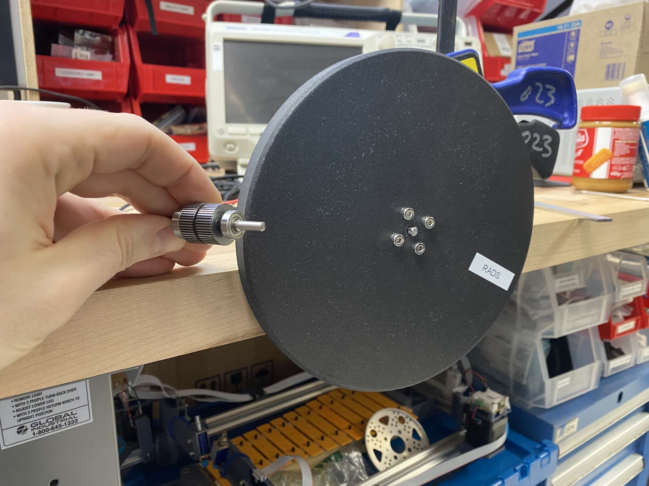
The motor’s own rotor has some inertia: for this tiny NEMA14, that’s about 0.000001878 kg m^2. Because this is so small, it was nearly impossible to get meaningful data for a model fit (although I did try): the rotor accelerates to its no-load speed in about 10ms, not enough time to gather very many samples. I bolted this giant PLA disk on (0.002888 kg m^2) to slow things down.

As an interesting aside, a common rule of thumb for motion systems design is to pick an actuator whose reflected inertia is about equal to the inertia of the component it is pushing around. The inertia that I printed to make sampling simpler is ~ 1000x bigger than the actuator’s rotor.

Spin-Up Data and Filtering

To fit the rest of the parameters, we want to make some time-series data of the system operating and then fit that to a model. For this, I put the motor in direct_q_current mode, where we can just tell it how much current to try to put on the q axis. Then we just… swing it around: apply maximum torque in one direction, wait for about ten seconds, and then flip directions, waiting for another 10-or-so. All the while we are sampling a set of the motor / controller states and stashing them for analysis.

Data collection is simple - I just spin a known inertia around using maximal applied current, flipping directions after some number of seconds and taking a few passes in either direction.

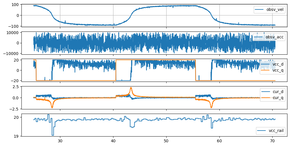
Time-series data from the test spin-ups. Note that while vcc_q moves rail-to-rail, the amount of current it generates is highly dependent on the rotor speed - this is back emf in action. Also interesting is to watch the vcc_rail signal (bottom trace): this is the power supply sagging when we pull current (it’s a USB-PD brick…).

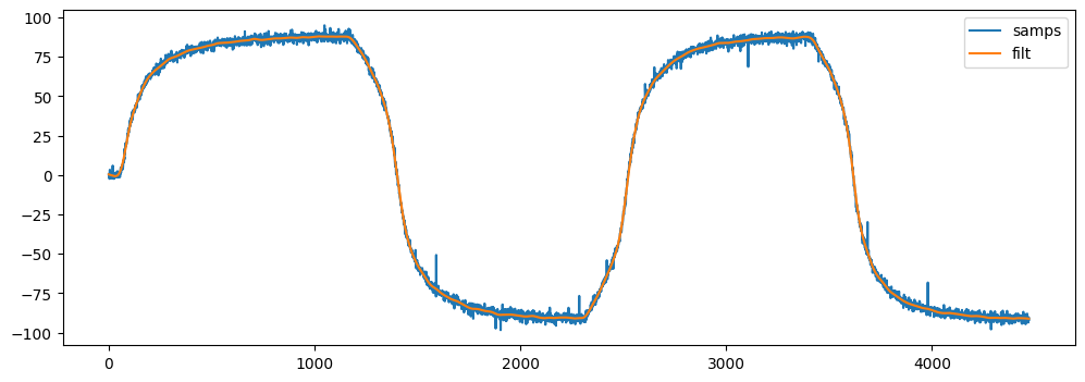
The observer’s velocity estimate is noisy (and it’s acceleration estimate is almost useless), so I filtered velocity using some newly acquired scipy magic.

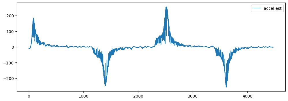
Once it’s filtered, we can take a discrete derivative of the velocity estimate to get acceleration data. These are still a little noisy, but serviceable.

We do a little filtering, etc (thanks scipy!) and then we can basically plot accelerations vs. speed, i.e. in ‘torque-curve’ land.

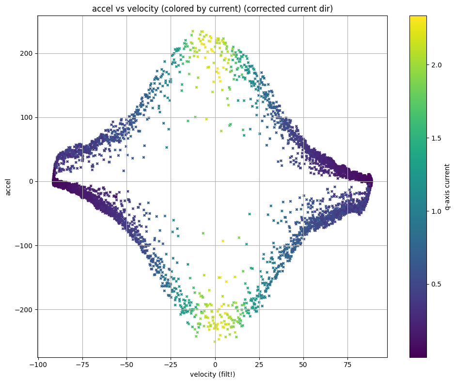
Looking at data from the spin-ups w/ velocity (x) and accelerations (y), with the rotational symmetry because we are spinning in either direction.

Fitting

To fit this, I’m just using scipy’s built in optimizer. We write a model with some params, then provide it with data and a loss function and if things aren’t too hairy it tends to work pretty well.

R = 6.8                 # ohms
J = 0.000001878         # kg m^2 (rotor) 
J = J + 0.00361 * 0.8   # adding le-diskus, plus print density ... 

def model(params, vcc_app, vel_now):
    ke, kd, kt = params 
    # assert that ke works against us regardless of speed dir. 
    ke = np.where(vel_now > 0, ke, -ke)
    cur_now = (vcc_app - ke * vel_now) / R
    acc_now = (kt * cur_now - kd * vel_now) / J

    return cur_now, acc_now 

def loss(params, vel_data, cur_data, acc_data):
    # hmmm 
    cur_guess, acc_guess = model(params, 20, vel_data)

    alpha = 0.0
    w = 1.0 + alpha * np.abs(vel_data)

    cur_error = np.square(cur_data - cur_guess)
    acc_error = np.square(acc_data - acc_guess)

    return np.sum(cur_error + acc_error)

# outfit an initial guess 
params_x0 = [0.001, 0.001, 0.001]

# run the minimizer, from scipy.optimize.minimize 
res = minimize(
    fun=loss,
    x0=params_x0, 
    args=(vel_data, cur_data, acc_data), 
)

I had also tried a scheme where we reshape the data into input and output states across time steps, then use the optimizer to tune variables so that an ODE of the system would correctly predict the next step, but I found that pretty ineffective, which is a shame since it’s a cleaner way to articulate dynamics in-general.

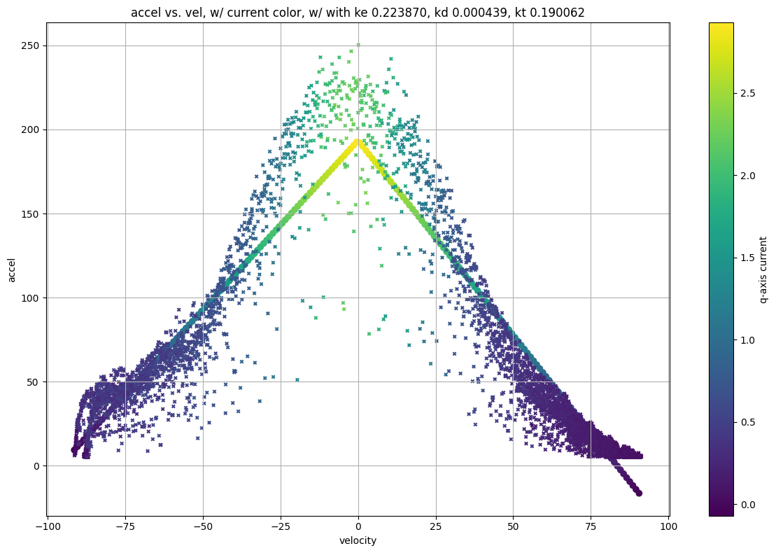
A fit! Although some wisdom says that k_e and k_t are equivalent, I let this model fit them independently because I suspect that in this case k_e also captures losses due to phase lag in the commutator - i.e. at high speeds the q-axis is not exactly aligned with the rotor’s real position.

What’s up with the Mismatch ?

There’s obviously a lot missing in the model. What initially confounded me is that the model suggests that when the applied voltage is positive but velocity is negative, (or vise-versa) we should see much more torque, since the effective voltage is greater with EMF working ‘with’ the power supply: \(V_{effective} = V_a - k_e (- \dot{\Theta})\)

The big mystery to me is how the power supply acts when faced with regenerative loads. For these tests I was using a USB-PD brick with a decoy, which is probably a sin in power electronics. In the data traces where I measured supply voltage during the tests, it doesn’t change meaningfully during these reversals (although it does dip when we use lots of current). In my understanding, even regenerative power supplies will only increase the supply voltage marginally during regeneration, doing so to drive current back into a battery (or dumping it into a resistor), so the back half of this plot should at least be flat.

I suspect a few things are happening here:

(1) The commutation speed is not fast enough to keep up with high angular velocities, so ‘on-axis’ current as measured is not totally on-axis, since the rotor’s electrical angle changes so quickly. This is especially true for a stepper motor, where we have 50 electrical rotations in each mechanical revolution. On the scope, I could see instances where one electrical rotation occurred over the course of only four or five PWM cycles.

(2) There are lots of losses that aren’t modeled here. Motors make a lot of heat in the form of \(I^2R\) and we also heat the stator and rotor iron as we spin it through the magnetic hysteresis loop. This is probably the most obvious contributor to the fact that the output torque drops off irregardless of the sign of speed w/r/t the sign of the applied torque… most of the power in these states is consumed by simply swinging the magnetic field around, rather than turning into useful current. I think on this front I need to understand the motor-as-an-inductor’s frequency dependent impedance… that pesky inductance - actually it is staring at me right in the face: \(V = IR + L\dot{I}\) - the term I didn’t stick into this model.

(3) The motor may be saturating its magnetic field. Current is equivalent to torque so long as we haven’t reached saturation, but the relationship is nonlinear once we are making lots of field meaning that as we drive higher and higher currents, torque stops increasing. IIRC most magnet steels saturate around 2.0 Tesla of field strength - this is one of the fundamental phyiscal limits to electric motor performance (and transformer performance!). This might contribute to the fact that the torque seems to ‘level off’ around zero velocity (i.e. is bell-shaped).

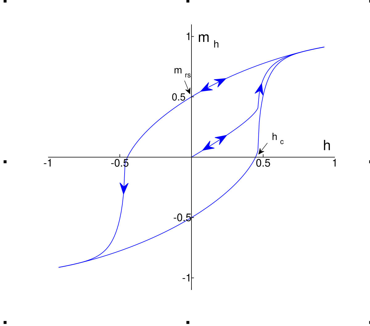
Via Wikipedia, also see Encylopedia Magnetica. The magnetic hysteresis loop - magnetization (m) is related to field applied by an electromagnet (h), but saturates when h is big. The area inside of the loop represents loss.

So, modelling is hard and the physics become complicated once we really dive into it. I think it is cool at least to be getting data at this point, and fitting some simple models, although I am weary to trust them too much.

To continue testing and learning, I think that I should more carefully monitor the power supply’s behaviour. USB-PD bricks are obviously not meant for this kind of thing, and I was hardly even using that much bypass capacitance in these tests.

I also suspect that losses and winding impedance at higher frequencies are the primary missed-model-components here, so I should endeavor to model them next.

I should also check to see what the effect of changing the drive mode is in the hbridges: at the moment, when the applied voltage is ‘off,’ current is allowed to recirculate in the low-side of the bridge. In prior controllers, this was different - ‘off’ time used a fast-decay mode. It might be the case that fast-decay is advantageous when we are slowing down, and recirculation is better when we’re accelerating.

Finally, I should try to improve the commutation speed. Using the observer, I should be able to update the rotor’s position estimate more often than I am able to sample the encoder - which I am already polling as fast as that hardware allows me too.

Measuring Torque + Trajectory Following

So far, none of this is actually directly useful to me, besides being a really great learning exercise. As soon as I realized how difficult it would be to tune good PID gains for the motor (esp. since changing dynamics…), I was trying to think of a way to measure active torque while running in open loop, since that control mode is so dead-nuts simple, and the PI gains for the current controller are at least easy to tune if we know the electrical values (R, I) which in this case we can get from the datasheet.

In practice, I have machines with ~ 8 motors total, and tuning gains for each of them remains too-difficult to be worth it, especially since open loop steppers already work well enough - instead, I want to be able to use these motors to make models of the system so that I can i.e. intelligently tune my lookahead controllers, i.e. set maximal accelerations and speeds.

Here, the motor is following an open-loop s-curve trajectory generated with my motion controller. It’s using the current controller stage for this, and reading the encoder just to ascertain how much of the current is on the d-axis (in blue) vs. on the q-axis (red) (y-axis is scaled incorrectly, whoops!). Only current on the q-axis is responsible for generation motion, the rest is waste - this is typical of a stepper motor. The oscillation in both signals comes from the motor’s rotor ‘springing’ around to align with the magnetic field.

For a while I thought this would require the position controller, using the output from that controller to measure how much ‘effort’ was required to move the motor under certain tracking conditions - but really it is pretty simple: we can always measure on-axis current to know how much of it is actually responsible for moving the rotor around.

  // in controller.cpp, current control loop 
  case CONTROLLER_MODE_CURRENT_FOLLOWER:
    {
      // we track active currents w/ the rotor-tracking projection, 
      active_dq_currents = lut_trig_xy_2_dq(enc_2_elect_phase_latest, active_ab_currents);
      // but we control current on a target angle that is moving in open-loop, 
      // following our interpolator blindly... 
      follow_dq_currents = lut_trig_xy_2_dq(follower_target_angle, active_ab_currents);
      active_dq_voltages.d = pi_d_axis.run(follower_d_current, follow_dq_currents.d);
      active_dq_voltages.q = pi_q_axis.run(0.0F, follow_dq_currents.q);
      // transforming that back and writing voltage / pwm as usual
      active_ab_voltages = lut_trig_dq_2_ab(follower_target_angle, active_dq_voltages);
      hbridges_write_pwms(active_ab_voltages.a * HBRIDGE_PWM_REQ_MAX, active_ab_voltages.b * HBRIDGE_PWM_REQ_MAX);
      break;
    }

This is fundamentally the same to any other open loop stepper driver / controller, but we are leveraging the FOC hardware to generate a signal that we can use to see how much force is actually being exerted on the system. The modeling above, also, helps us in setting our feed-forward parameters like maximum acceleration and velocity… soon, I’ll also be able to write about how I’ve been using those models more completely with a model predictive controller deployed for lookahead planning on a machine system.

What’s Next

Well, I set out to make a controller that could turn (almost) any stepper into a high performance servo - a goal shared by many - but I spent most of the allotted time in the nuts-and-bolts.

I’m glad to understand the problem a little more in-depth, and to have seen all of the gains we have to tune:

• the encoder calibration
  • done, reliable, repeatable, and easy to sample
• current controller PI gains
  • easily done with known R and L, but somewhere beyond my current comprehension
• observer alpha, beta, gamma gains
  • should be purely functions of the present noise, but hand-tuned for now
• position PID gains
  • a strong function of the motor’s context
• model kt, ke, and kd
  • made a reasonable fit, but clearly missing the inductor’s impedance

So I would say that at this point I have learned where all of the problems are, and where the holes in my understanding lie - honestly a great success. I would dive back into the impedance issue right now, I think having figured it out as I wrote all of this down, but I have to get back to the main activities.

I have also been thinking a lot about how to hook this up to the rest of my motion controller. In my machine systems, I stream splines to motors using a fixed point represtentation and a basis spline (aka b-spline) formulation. These have been really productive, and they have the nice property that we can use them to evaluate not just position, but also velocity and acceleration at any time (within a window of available control points).

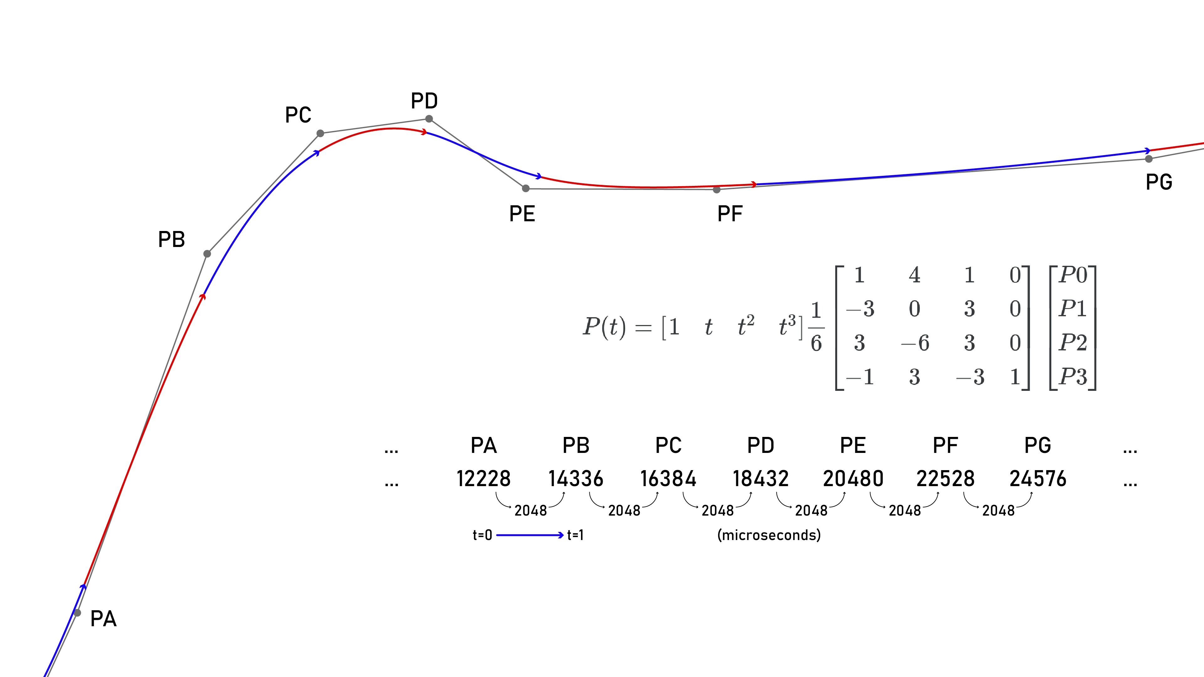
I commonly use basis splines to transmit trajectories from planners to motors. \(P(t)\) is position as a function of time - the first, second and derivatives are also well defined: velocity, acceleration and jerk.

I saw a note recently on feed-forward terms in position controllers like this one, which is that it’s productive to feed forward some gains from a trajectory’s acceleration and speed curves.

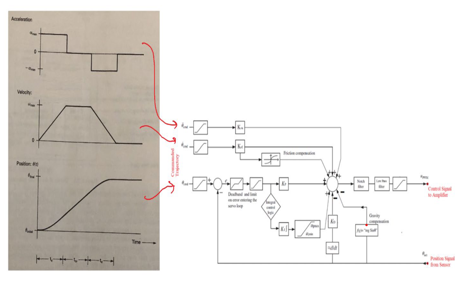
Via app note 103 / 102 from Oracle Robotics - shows how acceleration and velocity terms from a known trajectory can be fed into a position control loop - it also notes a gravity compensation term (towards bottom right).

The splines obviously provide a handy set of accel and velocity values to feed-forward, and the gains I would bet we can find using a more complete motor model and some knowledge of the inertia that the motor is working with… it might even be productive to try an LQR controller with multiple inputs (target accel, vel, pos), rather than i.e. the PID with feed-forward gains.

I also have lots of work to do in the firmware to i.e. remotely write encoder tables, and work to do in the calibration scripts to integrate it all into one or two steps: plug in a board, get the encoder table, run some tests and fit the rest of the system. Then there is the question of how to cleanly represent all of that to higher level motion planners.

For a litmus test, I would like to verify the torque measurements with calibrated loadcells - one of the knuckles boards is a CS5530 loadccell amplifier that can run up to 4kHz, it would be awesome to see time-series of the motor in action reporting torques and compared to direct measurements with one of those.

So! I have probably just scraped the surface on this one. I should endeavor to graduate soon and become free to work more intensely on these things; I would really love to provide high-quality, closed loop, comprehendible open source motion control systems that are easy to use… soon!