Deployable robots in the woods!

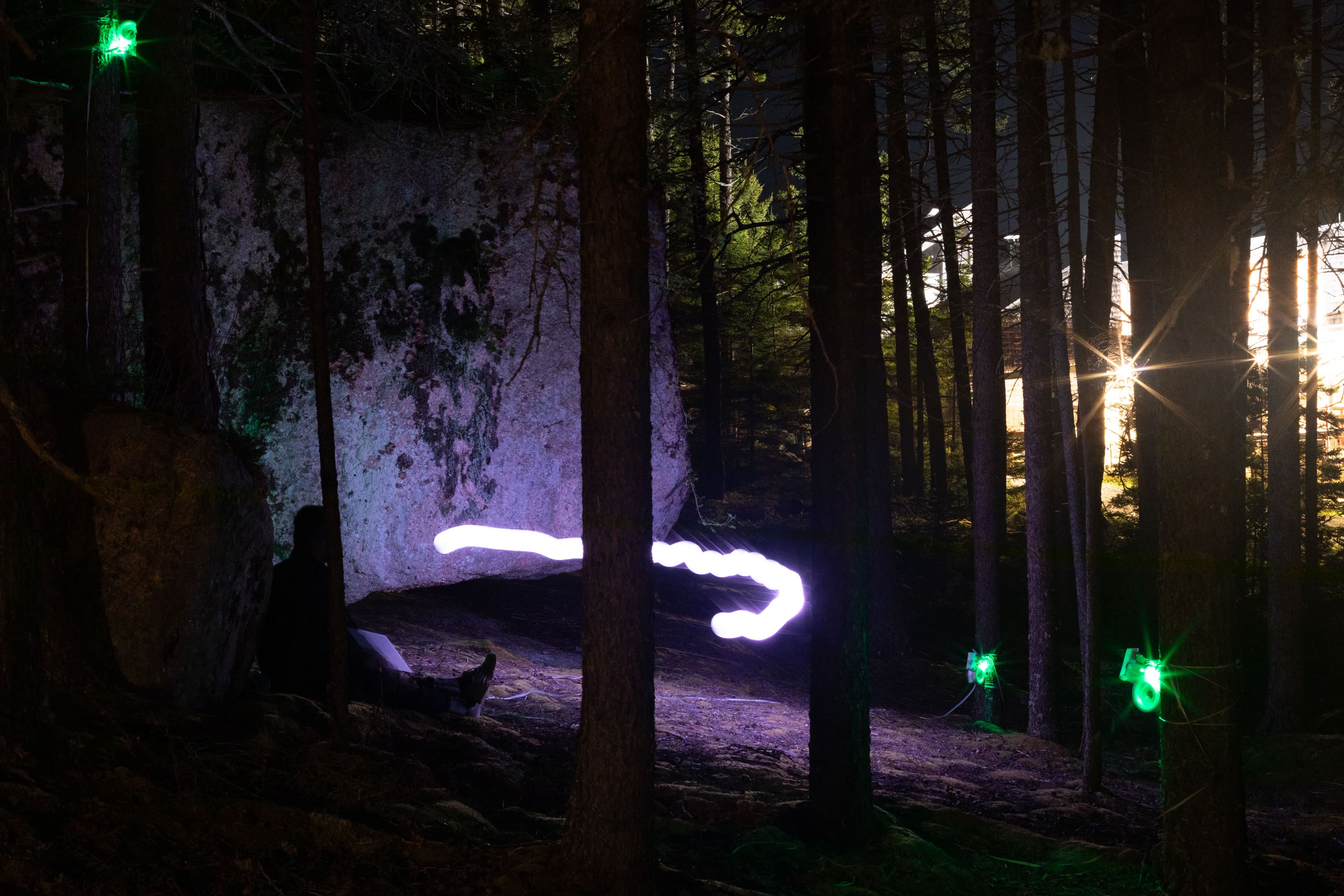
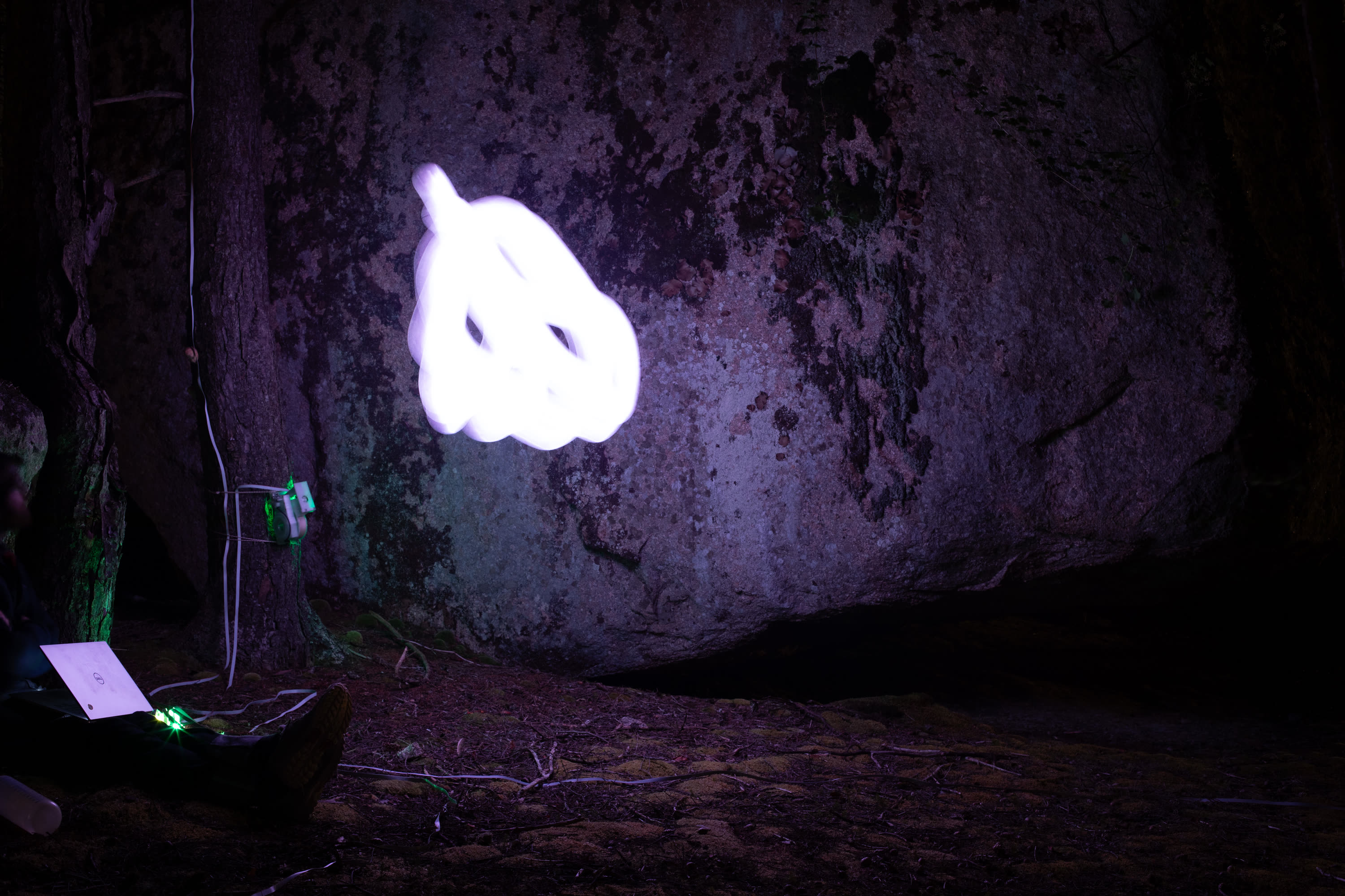
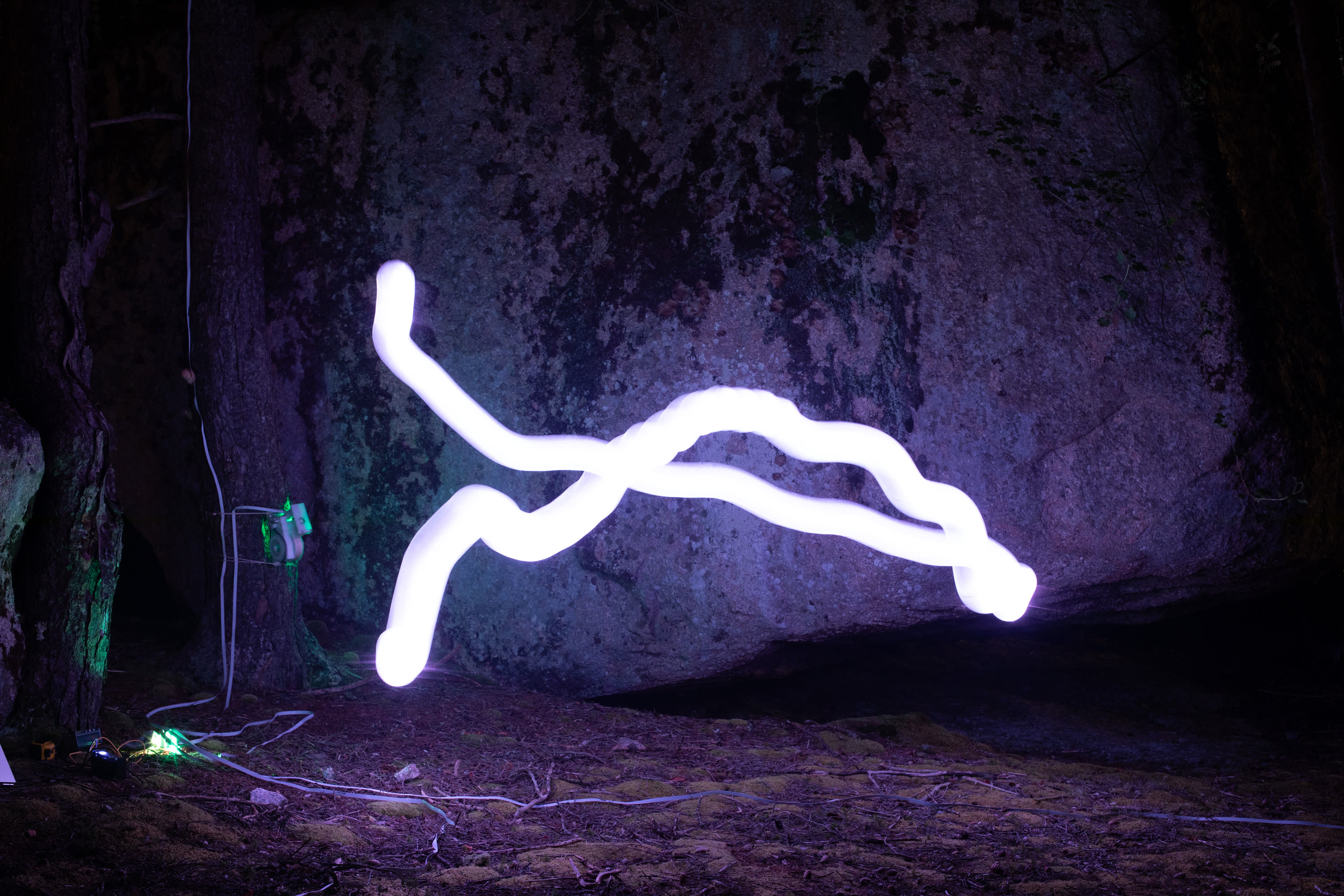
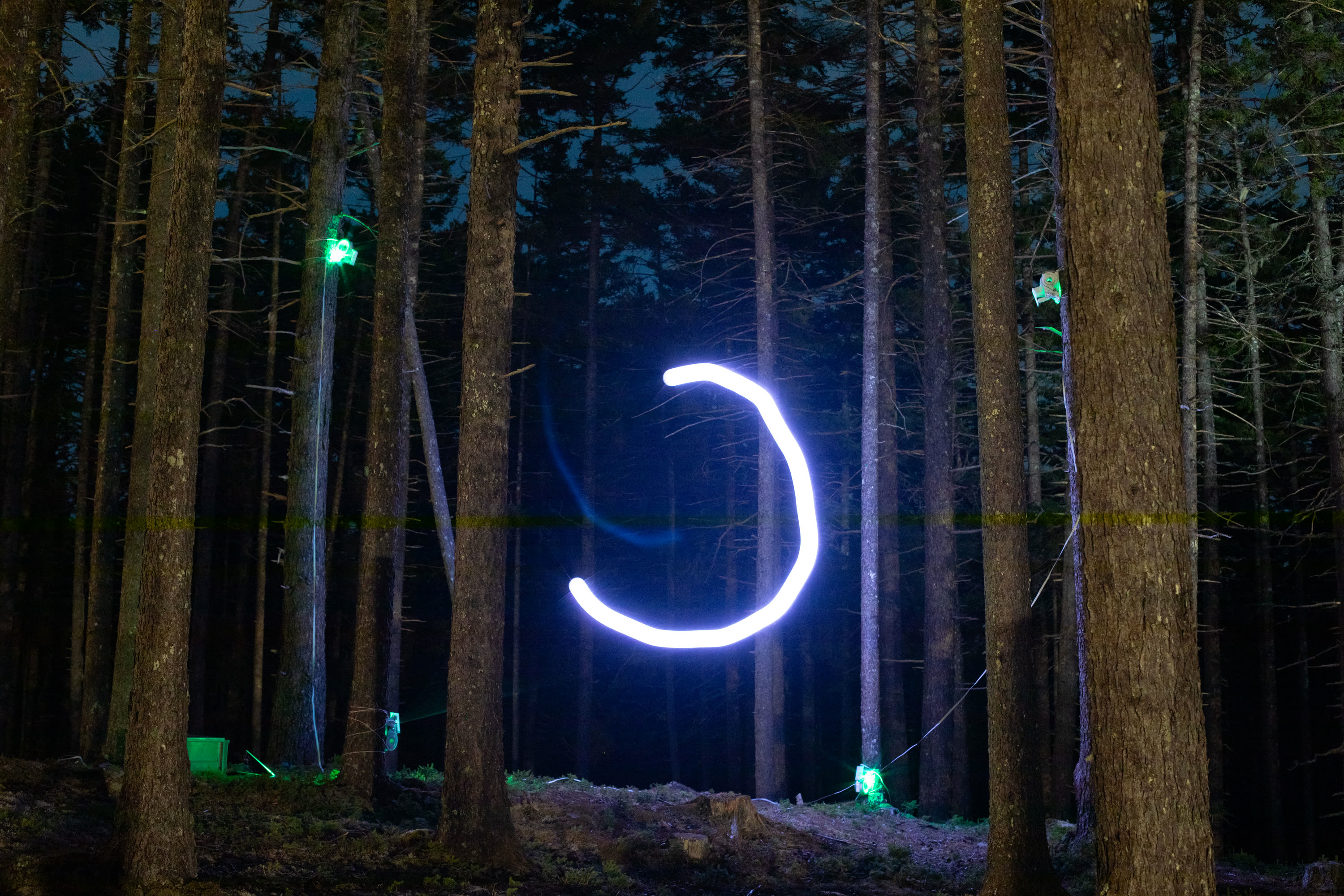
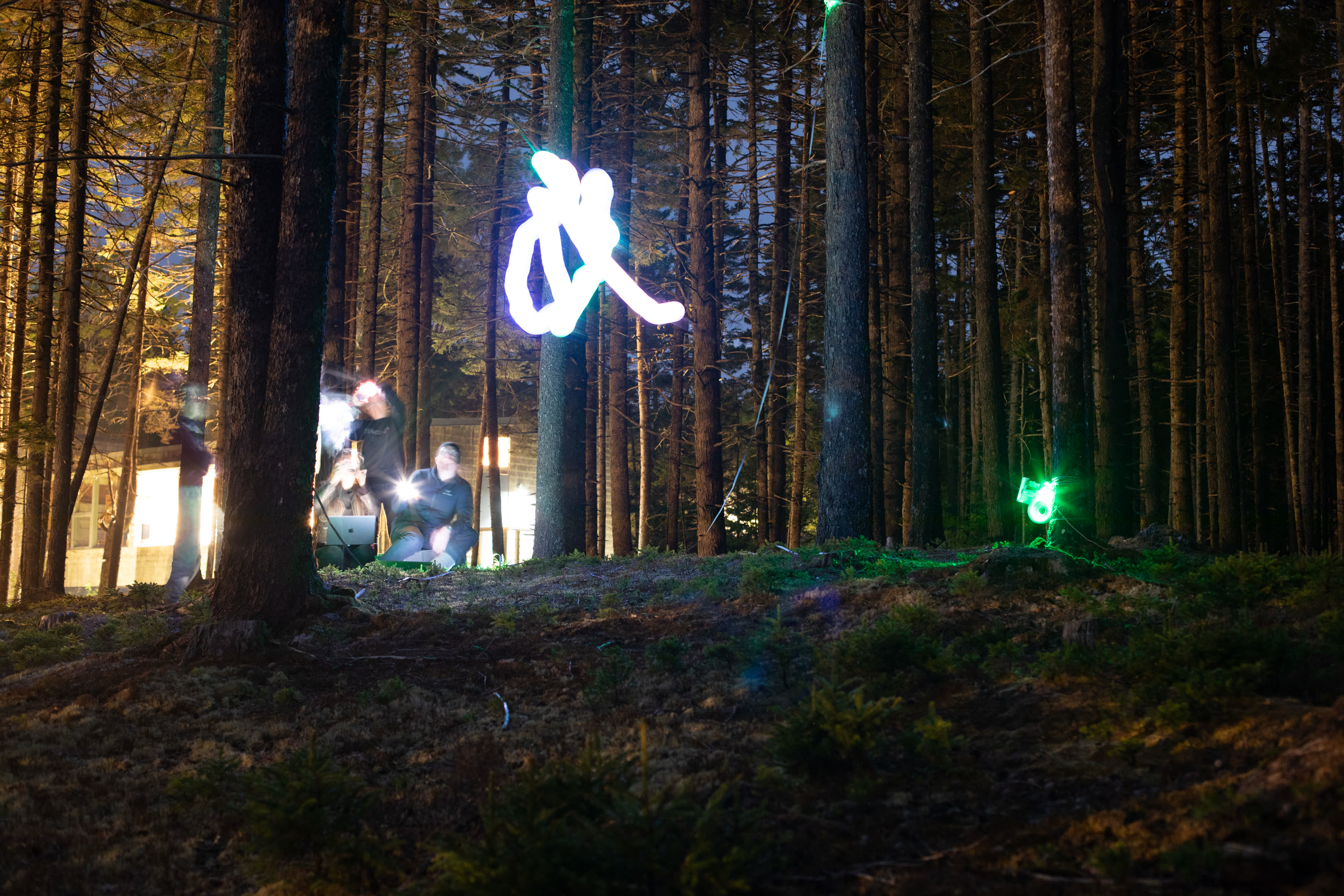
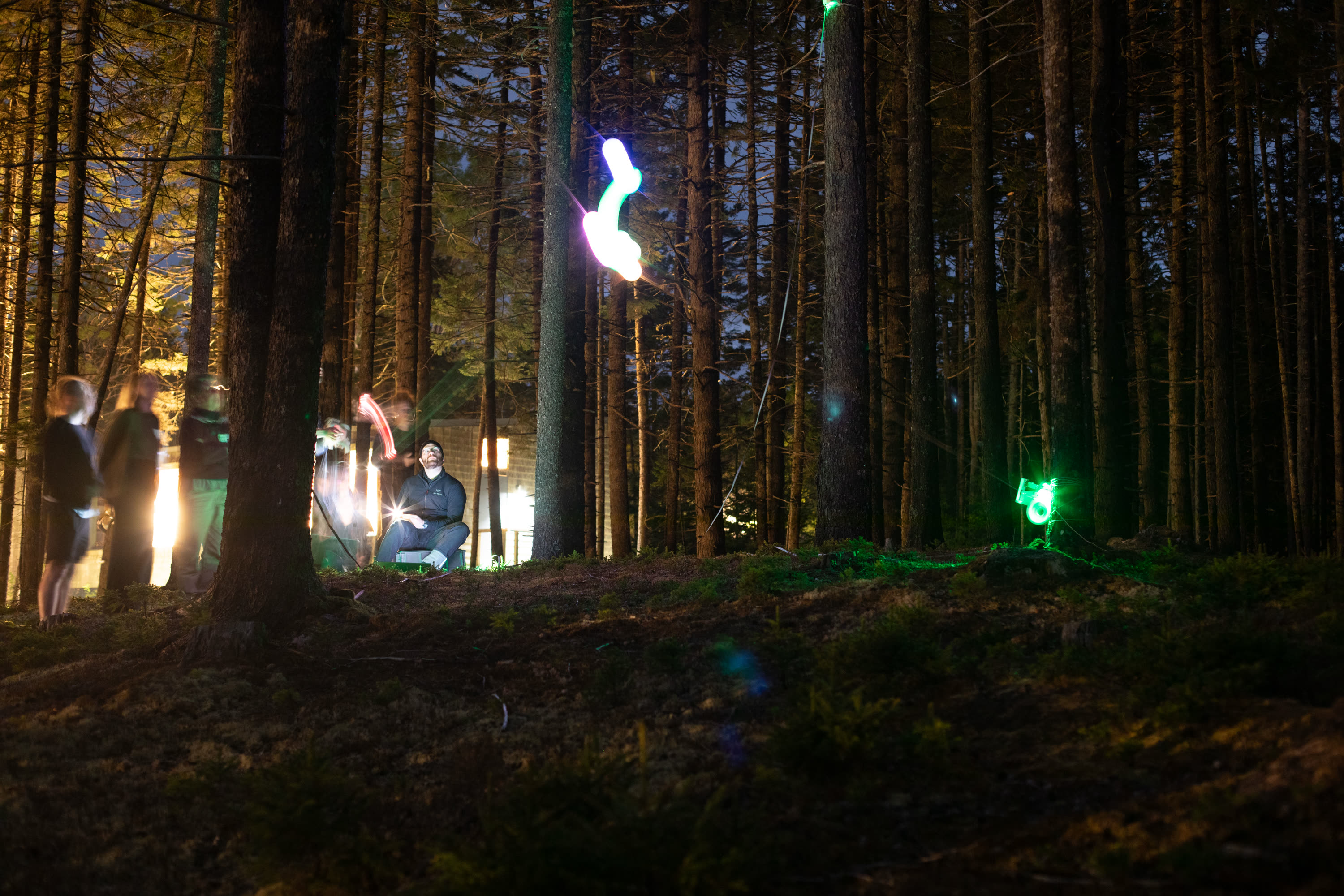
Drawing in space!

Long exposure linework.

I got lucky again this year and was able to join in Haystack Labs, which is a craft school / summer camp that Neil (my advisor) and James Rutter (Haystack Fab Lab Director) temporarily repurpose (for six days) as a kind of craft x digital-fab experiment. The gist of the experiment is to ask: why is it that digital fab and craft seem mostly like oil and water, and what can we do to emulsify them?

I think that mixing craft and digital fab is a kind of generational task… many of my favorite collaborators and advisors (Ilan Moyer, Leo McElroy, Nadya Peek, and Quentin Bolsee) are making big contributions here. I have always hoped that my own work will contribute along this front, making it easier to make interactive tools with human-and-process feedback across multiple levels, but for all of my efforts, the tools I have developed have yet to hit the level of reliability and usefulness that they would be appropriate to deploy in these messy environments. I have resolved that I will have to leave grad school and gather a team in order to fulfill that dream.

It was my fourth time at Haystack - in the past I have made a clay 3d printer and another one… and this weird pots-and-pans machine. This time around, I decided to try to build something wondrous - to do machine building as a craft, in a shamelessly self indulgent way. Art, babey… and the simple joy of making things that move.

What / Where

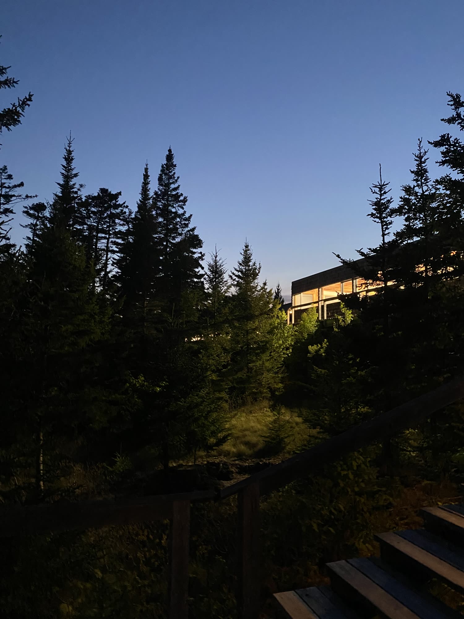
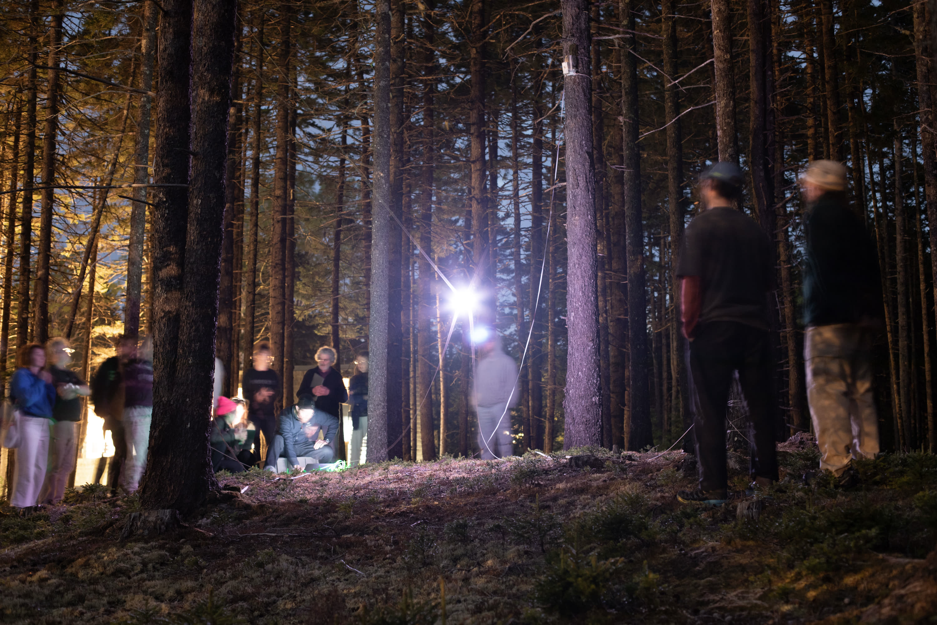
Haystack is a gorgeous place: the coast of Maine, an island reachable via an island, and woods, moss crawling over rocks. I was programming in the woods and it was joyous.

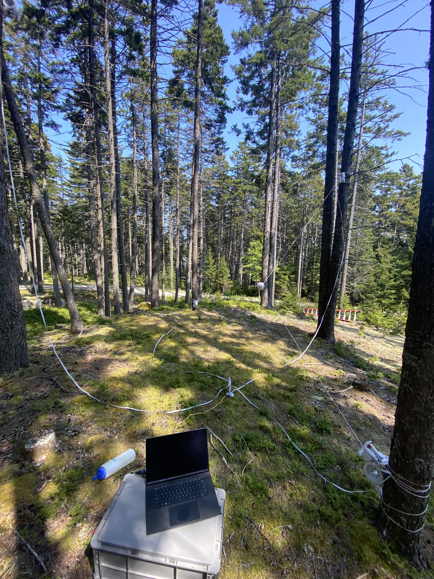
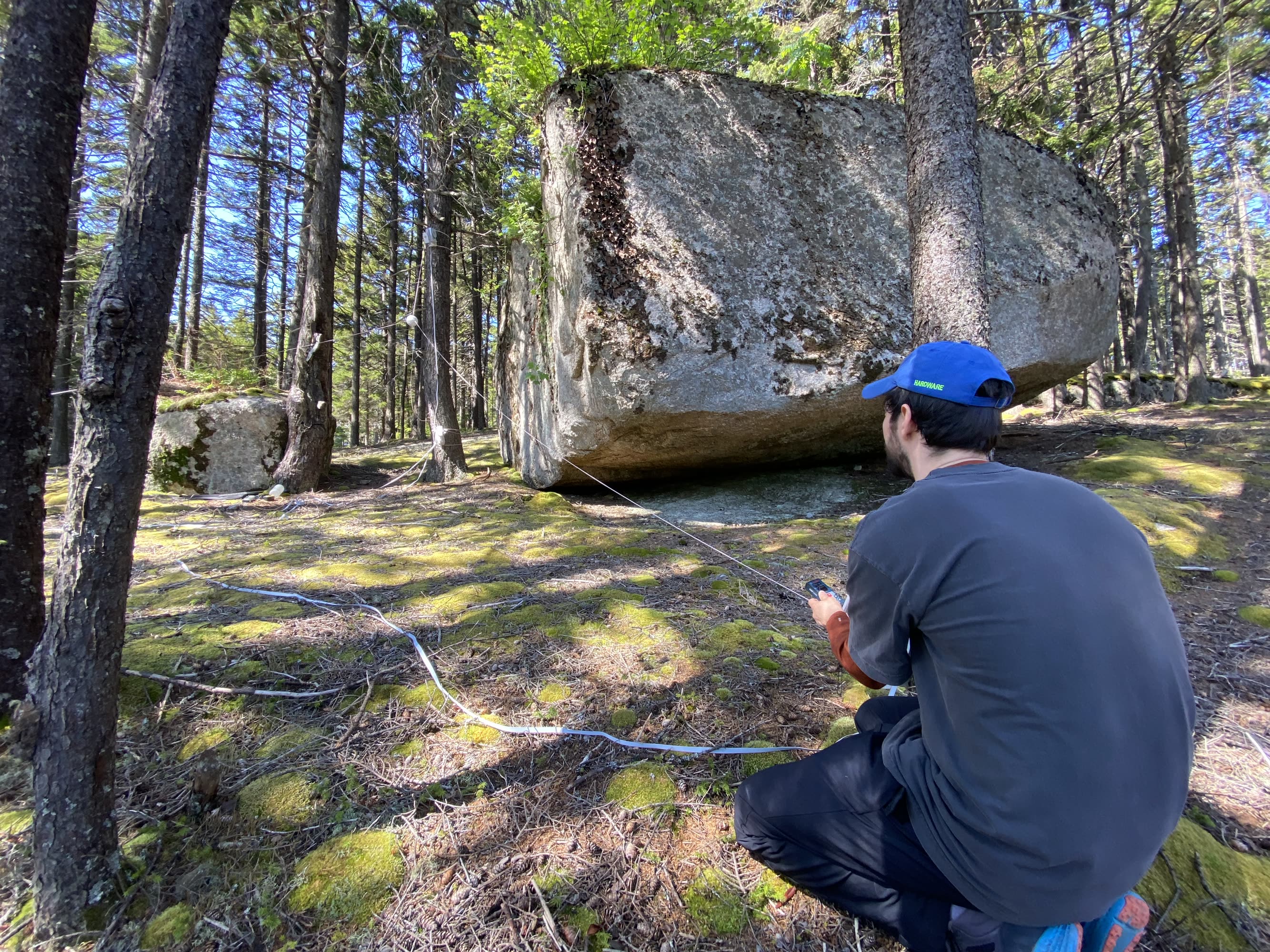
I wanted to make a machine that was lightweight, that we could install in an hour or less, and take away with no footprint. So: the winches.

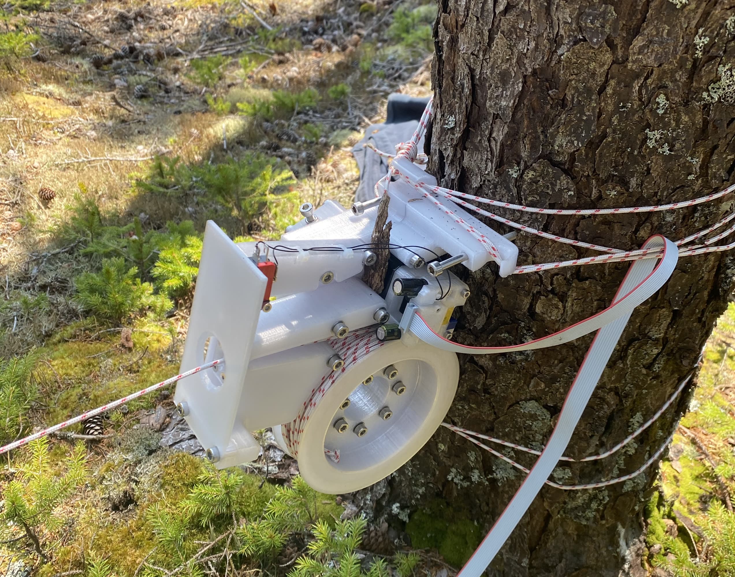
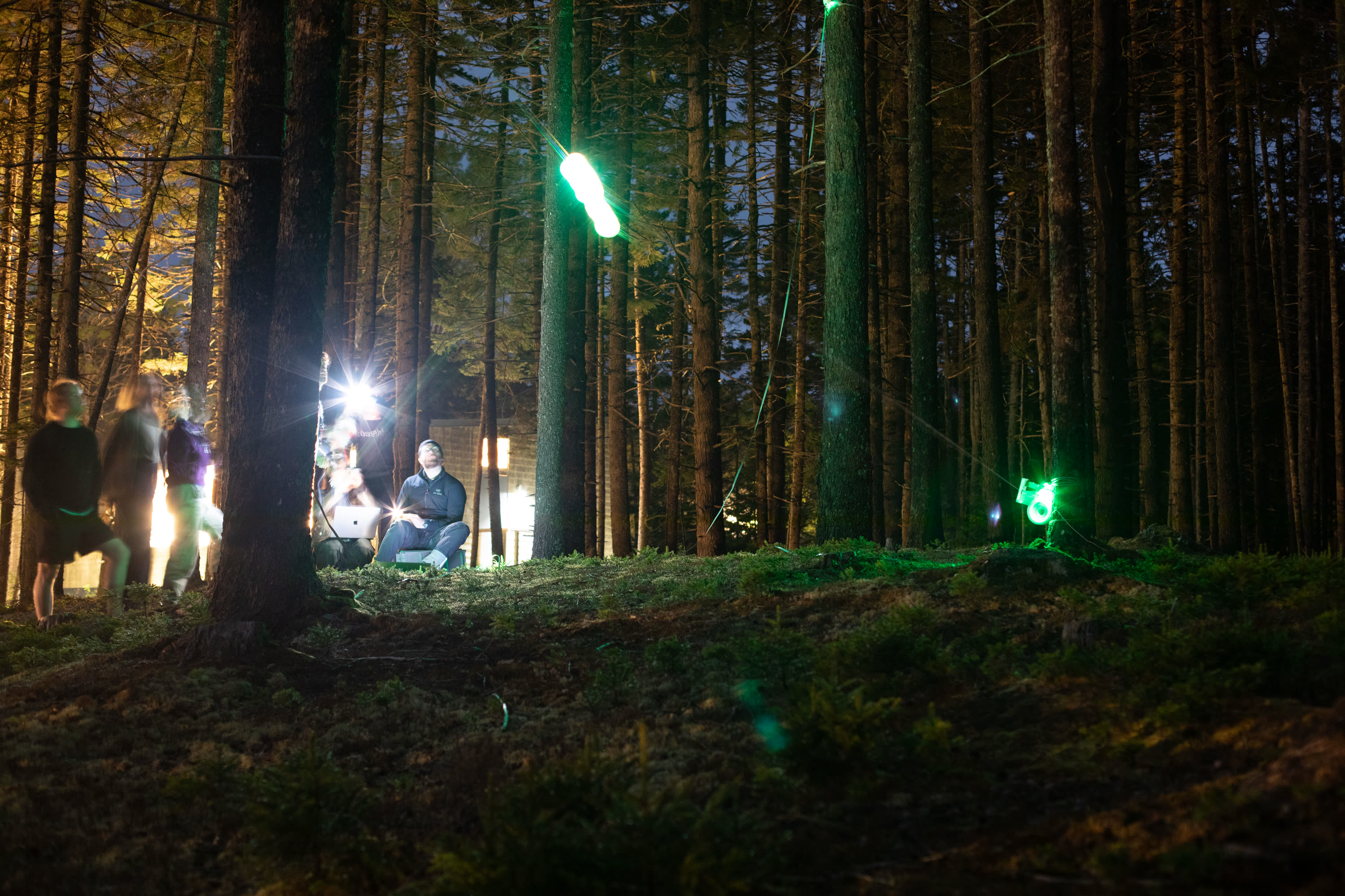
One such winch, lashed to an unsuspecting tree.

I made four of these: torque-controlled winches that use my latest driver, and one of my favourite design patterns for a belt reduction. The spool does not have any ‘tending’ hardware, i.e. the rope simply winds on, so we can’t be completely sure what the exact diameter is at any given moment (not good) but the thing is pretty coarse anyways, so I eschewed the complexity that would have entailed.

Rope enters the spool through a small teflon o-ring, so that the angle of entry doesn’t change the friction too much, and this entrance (… known colloquially as the butthole) is positioned about 150mm from the spool, in an effort to have the rope coil up nicely on the spool.

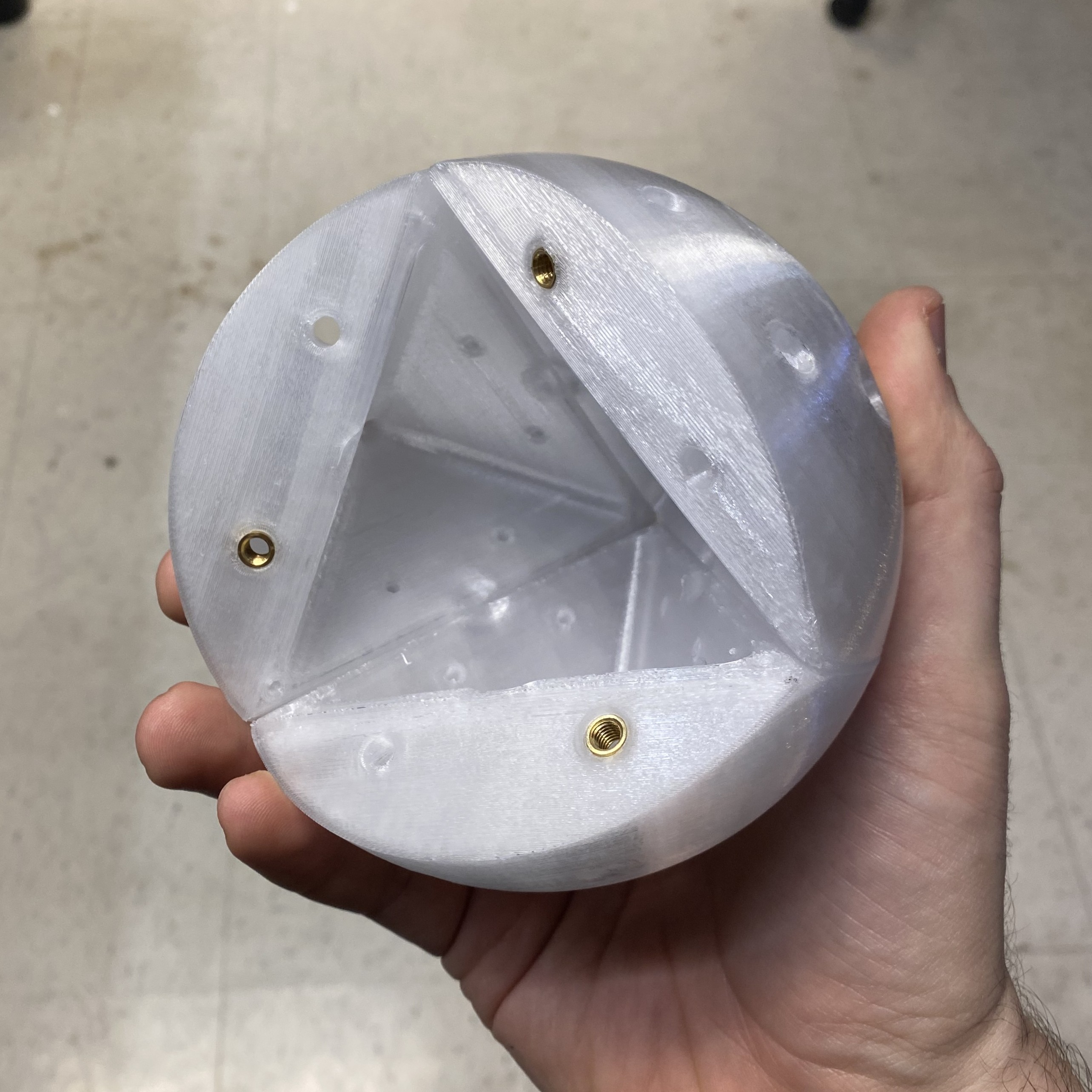
I also designed the orb - a sphere with four entry points, and interior mounts for some RGBW LEDs. We stuck an ESP32 in here and a 21700 LiPo cell, so that we can change the light’s color and intensity remotely over WiFi.

There’s a flap on each winch with a limit switch, which we use to home the machine… this little bonk might be my favourite part of the whole project.

The homing / geometry discovery sequence: last three motors are shown.

The orb has a ~ spooky ~ vibe, hence the Blair Winch...

Homing, and Learning Where the Winches Are

Credit goes to Quentin for figuring out how this should work, and implementing it in a routine that I could plug into the controller.

Homing the winches is simple-ish: we startup each motor, and then run them sequentially with three (idling motors) under some minimum torque (to keep lines straight), and the fourth (reeling motor) at a larger torque. Then we pull motor encoder measurements (which we can correlate to rope lengths), as the chosen motor reels the orb in towards the limit. Once that limit is hit, we swap motors so that the next is reeling and the rest are idling. We do this four times, so that each motor is the reel-er once.

After the homing routine is done, we have a big system of equations to solve. The main issue it that we don’t know where the winches’ rope-entry points are, we’ll call those \((w0 \ ... \ w3)\). At each time step in the homing routine, we have rope lengths (measured) for each winch \((r0_t \ ... \ r3_t)\). We also add a long list of unknown positions of the orb for each time step, \((orb_t)\)

We assume that at each time step, the distance of the orb to each winch is matched to the measured rope length… i.e.

This gives us a pretty simple loss function: for each time step, some \(orb_t\) should exist that is \(ropeN_t\) distance from each \(wN\) position. If we apply that loss to each time step, we find \(wN\) positions that are consistent through time (… the winches don’t move). So, sort of oddly, to solve for the winch positions we also have to figure out what the whole homing trajectory looked like.

This is a simple loss, but there’s lots of data - normally 1000 or so points along the homing trajectory. So we throw that over to scipy.optimize.minimize to chew through it.

count = 0

def loss_func(x, data):
    global count

    n_motor = 4
    tot = 0
    n = len(data)

    # winch positions
    xyz = np.reshape(x[:n_motor*3], (n_motor, 3))

    # orb positions: one for each time step 
    p = np.reshape(x[3*n_motor:], (n, 3))

    # guess is good if distance from winches to the orb 
    # matches the measurement at that time step 
    for i in range(n_motor):
        dist_sq_i = np.sum((p[:, :] - xyz[i, :])**2, axis=1)
        err_i = np.sum(np.square(dist_sq_i - data[:, i]*data[:, i]))
        tot += err_i / (n_motor*n)

    count += 1
    if (count % 1000 == 0):
        print(math.sqrt(tot), flush=True)

    return tot

In the end, this solved pretty well each time we ran it. I stuck it in a subprocess so that we could run it (takes a few seconds) after the homing routine, with the rest of the controller still alive and talking to hardware. The solver doesn’t solve in any fixed orientation (although we tried that), instead it just orients the solution randomly. Once the hard part is done, Quentin simply rotates the solution around such that w1 is at 0, 0, 0 and the vector from w1 -> w3 is vertical along z and w2 is somewhere in the XZ plane. Good enough for a first pass, probably we could also look at torques over time to ascertain the z / gravity vector, but not today.

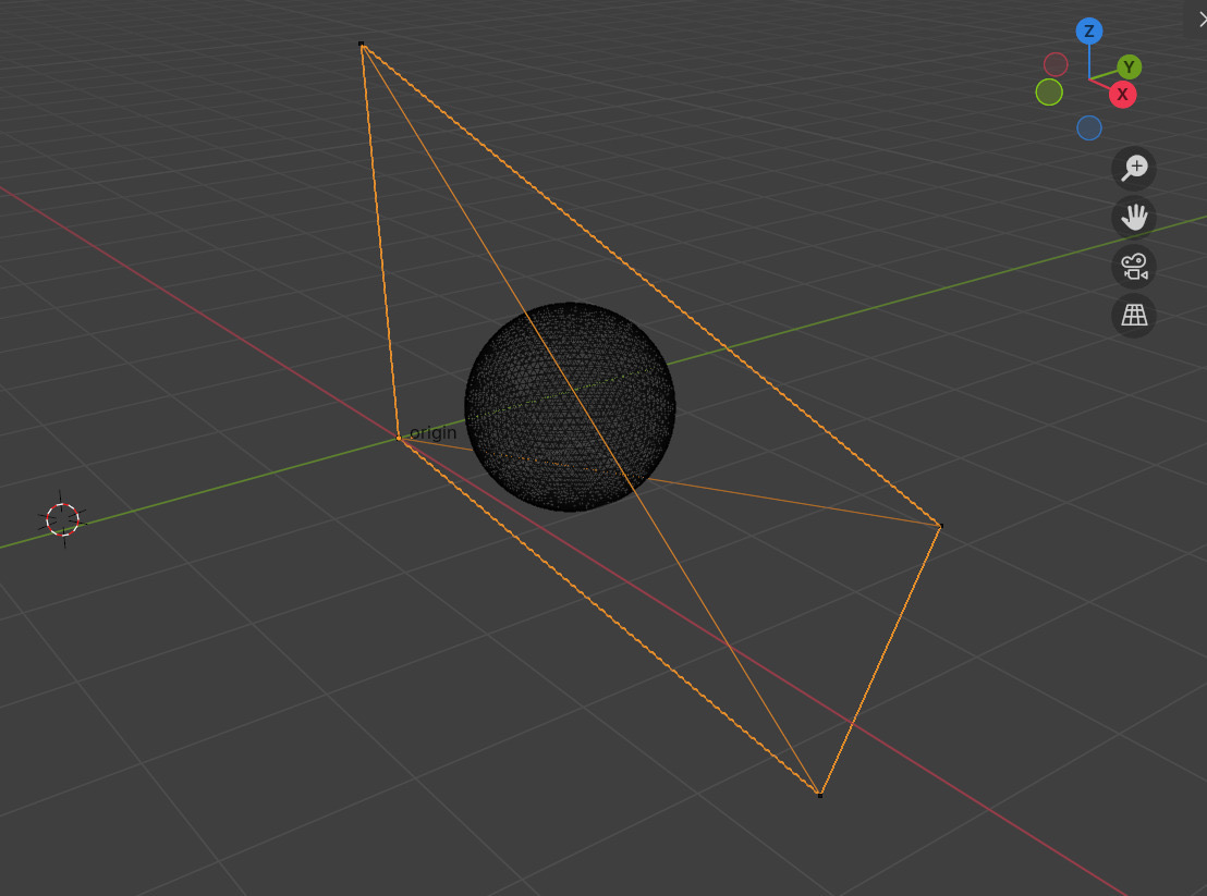
To get a qualitative check for the solve, Quentin popped output points into blender, which let us check if the tetrahedron was ~ about the right shape.

The solver also returns the tetrahedron’s insphere radius and location, which is a useful place to move target trajectories into: points in the insphere are guaranteed to have relatively nice reachability, whereas i.e. points outside the tetrahedron are unreachable (obviously) and points close to the corners require using lots of torque on one of the motors…

With some help from Sebastian of morakana, we validated our tetrahedron solves by measuring vertex-to-vertex lengths.

An Aside: Solving w/ Unknown Offsets

As the orb approaches each of the stops, the geometry changes such that the opposing three motors exert more force on the orb: i.e. we are pulling “more away” from motors 0-2 when we are close to motor 3. This is obvious when you look at the geometry, and raises an issue with the somewhat underpowered winches: in the first setup we did, the tetrahedron made up by the winches was pretty far from an “ideal” tetrahedron… this made for a situation where the homing motor wasn’t able to reel the orb in completely. We tried initially so solve this problem away, by having our solver learn these offsets as well as the rest of the geometry, i.e adding an unknown offset \(roN\) …

Neither Quentin or I could get it to solve consistently. Probably it is possible, but it was beyond us at the time (although Quentin certainly got closer).

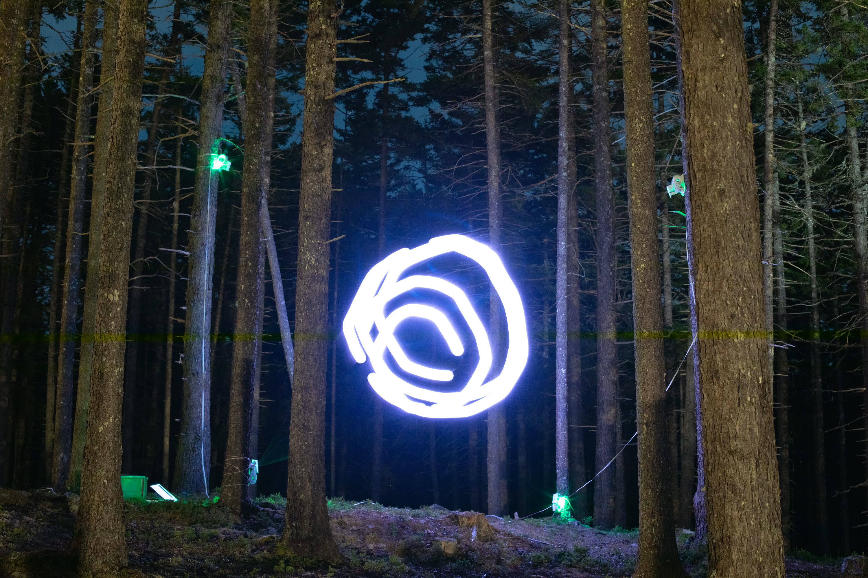
This shows the homing routine w/o offsets, where we flip motor directions once the orb has stopped for ~ 200ms. It should be possible to solve even with this data, solving also for the final offset in each direction, but that turned out to be a second-spiral task. This video also shows an attempt at control using only rope-length-setting output, which results in odd shaped circles due to the ~ nonlinear force that each corner of the tetrahedron exerts (and non-infinite torques).

To solve this problem ad-hoc styles, we added additional stops on the rope to make sure the limits were hit, and measured that offset manually. The second tetrahedron we made was also much more regular, so this problem went away (i.e. the orb actually hit the stop in each corner).

Controlling the Orb

If only I had internalized more of Gil Strang’s class…

Controlling the orb once we had the winch positions was more involved than I had thought. My first naive attempt was to simply take the target position, measure what the rope lengths should be at this target, and then run PID on the motor torques to hit that. This worked fine but did not produce very smooth motion, and led to some instability when the winch positions were not very well worked out.

I eventually developed a net force calculation, to push the orb along a particular force vector at each time step. This involves a few steps.

I did manage to get the orb more-or-less under control, here it is drawing a circle in space - slowly, surely…

1: Where is the Orb ?

We have a target position at each time step, and we have rope length measurements. To figure out where the orb is, we need to do forwards kinematics (actuators to cartesian). This can be solved using sphere intersections: each winch is the center of a sphere, and each sphere radius is the rope length. With four lengths, this is overconstrained, but if we just take a subset of the motors it is perfectly defined always (so long as all spheres intersect).

def sphere_sphere_intersection(c1, r1, c2, r2, atol=1e-9):
    """
    returns (center, normal, radius)  |  None
    """

    d_vec = c2 - c1
    d = np.linalg.norm(d_vec)

    # Degenerate centre-coincident case
    if d < atol:
        raise ValueError("bad circles")

    # No intersection if too far apart or one inside the other
    if d > r1 + r2 + atol or d < abs(r1 - r2) - atol:
        return None

    # Unit vector along the centre-to-centre line
    e = d_vec / d

    # Distance from c1 to the circle’s plane (along e)
    x = (d**2 - r2**2 + r1**2) / (2.0 * d)

    # Circle radius^2
    r_c_sq = r1**2 - x**2
    if r_c_sq < -atol:      # Numerical guard
        return None
    radius = np.sqrt(max(r_c_sq, 0.0))

    center = c1 + x * e
    normal = e              # already unit length

    return center, normal, radius

def fwds_kinematics(tetra_vertices, rope_lengths):
    # intersect 0, 1 to get a circle betwixt, 
    circ_0_1 = sphere_sphere_intersection(tetra_vertices[0], rope_lengths[0], tetra_vertices[1], rope_lengths[1])
    if circ_0_1 is None:
        # bonk, return center ... 
        print("sphere-sphere intersect fails")
        center, rad = insphere(tetra_vertices)
        return center 

    # intersect circle and third to get two points... 
    pts = circle_sphere_intersection(*circ_0_1, tetra_vertices[2], rope_lengths[2])
    if pts is None:
        print("sphere-circle intersection fails")
        center, rad = insphere(tetra_vertices)
        return center 
    
    if pts.shape[0] == 1:
        return pts[0]
    else:
        # pick tallest... 
        return pts[np.argmax(pts[:,2])]

I learned this trick while helping the HTMAA Architecture Group finish their machine. Works great.

2: Move the Orb

Once we know where the orb is, we can apply some force to take it where we want it to go. In this case, I simply chose a ‘requested’ force vector that was scaled with the orb’s current distance to the target: when further away, we ask for more juice, and when closer we dial that back. PID control, the quickest of hacks.

Then there is the matter of picking which motors to exert which torques. We know the orb position and the winch positions, we have four rope vectors that can exert some force (but only in tension), so we have to find a set of tensions that sums to the desired direction (and magnitude).

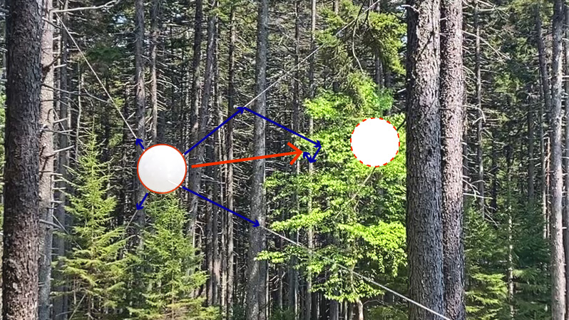
To control using ‘net force’, I calculate a set of tensions that best combine to produce some desired force vector on the orb. This would be simple if we could produce unlimited torques, but we sometimes don’t have enough juice to reproduce the desired vector exacly.

Were our motors infinitely torquey, this would always be possible - but they are not. To add complexity, we always have to exert some minimum tension to keep the lines taught (otherwise our rope length measurements get wacky).

I tried and tried to work this out using i.e. vector projections, but couldn’t quite nail it. I tried to summon my inner Gil but failed. Instead I used a least-squares fit that minimizes error to the target direction, ye olde have-someone-else-who-wrote-the-python-routine solve the problem for me: praise to the tools-builders, for they are truly His disciples! To check how much trouble this was causing, I calculate the resulting force vector’s alignment with the target at each step, and report that if it’s eggregious.

# net force vector style control 
def do_control_net_force_dir(tetra_vertices, rope_lengths, targ_dir, tq_min, tq_max, debug=False):
    pos_now = fwds_kinematics(tetra_vertices, rope_lengths)
    dir_vec = targ_dir
    dir_vec_mag = np.linalg.norm(dir_vec) 

    f_des = dir_vec       # desired Cartesian force
    f_des_unit = f_des / np.linalg.norm(f_des) 

    rope_vecs  = tetra_vertices - pos_now
    rope_units = rope_vecs / np.linalg.norm(rope_vecs, axis=1)[:, None]  # (4,3)

    B = rope_units.T            # (3,4)
    t0 = np.full(4, tq_min)     # initial torques (all @ min) 
    f0 = B @ t0                 # initial net force 
    f_res = f_des - f0          # extra force we still need

    hi = np.full(4, tq_max - tq_min)
    sol = lsq_linear(B, f_res, bounds=(0, hi), method="trf")
    delta_t = sol.x
    tensions = t0 + delta_t 
    # tensions = np.clip(tensions, tq_min, tq_max)

    # to check 
    # project torques back along ropes 
    f_final = B @ tensions
    f_final_unit = f_final / np.linalg.norm(f_final) 

    # angle betwixt ? 
    cos_ang = np.clip(np.dot(f_des_unit, f_final_unit), -1.0, 1.0)
    ang_err = np.degrees(np.arccos(cos_ang))

    # Magnitude error
    mag_err = np.linalg.norm(f_final - f_des)
    rel_err = mag_err / np.linalg.norm(f_des)

    # track max-latest 
    global control_iters, ang_err_max, ang_err_max_at
    control_iters += 1 
    if ang_err_max_at < control_iters - 100:
        ang_err_max = ang_err 

    if ang_err > ang_err_max:
        ang_err_max = ang_err 
        ang_err_max_at = control_iters 

    # compare torque result w/ desired
    if debug:
        print("do_control_net_force ...")
        print("f_des (unit)     ", f_des_unit)
        print("f_final (unit)   ", f_final_unit)
        print(F"f_ang_err        {ang_err:.3f}\t (max {ang_err_max:.3f})")
        print(F"f_rel_err        {rel_err:.6f}")
        print("")

    return tensions, dir_vec_mag 

I found that this caused lots of problems with tightly bounded motor torques (i.e. if the minimum torque is big, lots of trouble), but when I deployed more motor juice and controlled with smaller force requests, it was mostly OK. Next go-around I will either build stronger winches or write a smarter controller.

There is clearly lots of improvement here: we can always exert some amount of force in the target direction, and probably direction alignment should be prioritized over magnitude matching - i.e. the higher level controller (a p-only controller, hah), should avoid requesting forces that would require the direction vector to skew.

This controller doesn’t do any lookahead either, a clear flaw. I am working on MPC style controllers for other projects, and their utility here is clear, especially since the kinematics effectively changes at each time step. Modeling the orb as a mass in space (and gravity) would improve things, etc etc. I think it is a good test case, and I hope I will get to wake it back up once more to improve. For now, the output is satisfying:

MIDI -> Orb

Besides light painting, we also ran a little demo / concert with the gang at Haystack. Char plugged an accelerometer into strudel (a live-coding synth environment), and piped accelerometer values to the orb controller via MIDI. The values were also used to change some beat arrangements and samples… I transformed this data into orb motion, and people gathered-round for a try piloting the orb / music.

What We Learned, What We Missed

More Power == Better

Despite what I thought was a pretty solid belt reduction and reasonable sized NEMA17 motor, we were still torque limited in many cases. I think there’s lots of room to improve the controller to overcome this, but it would still of course be preferrable to be able to absolutely throw the thing around.

The upper limit wasn’t actually the motor (we only ran it near ~ 60% available output) - it was the belt, a GT2, which would occasionally slip on the drive wheel (which is printed…). Moving to a GT3, and improving the printed geometry would help in this regard.

Control with Smarter Limits

When the controller was in a position when it couldn’t exert a net force in the right direction, it would apply the best effort to hit the target magnitude / direction combo, meaning the thing would wiggle off trajectory. A controller that scales up to to maximum magnitude, without violating the target direction, might perform better - but then we would be running PID with a nonlinear real output. A smarter version of this would involve some more of that direction-vector modeling in the main control loop… MPC for the orb would be very cool.

Learning with Torques to boot

These motor controllers can learn parts of the motor model, and this project showed me pretty well where the next step would be: with a good motor model, we could also model i.e. the friction at the rope input (as a function of entry angle), and the winch’s stiction properties.

We could also add data to our solver by looking at net torques - i.e. if we keep rope lengths matched, then dial one motor up (more tension), and run a controller on the other motors to hold length, we get some information that describes the motors’ positions w/r/t one another, since we can assume the force vectors along the ropes in these cases are summing to zero. We would need to account for stiction there, too, but it’s all more data to better constrain the solver.

Learning All The Time

Something I’ve been really interested in is developing a controller that is continuously learning… each new time step generates a new set of rope lengths, motor output torques, and positions… we should be able to continuously add those to our data pile and occasionally re-run / improve estimates of the systems’ properties.

Very fancy versions of that system would learn also where they are underconstrained and then try to operate in regions where data is sparse, to better characterize the whole system… and with enough data, also measuring i.e. motor and driver temperatures, we might learn about how i.e. heat saturation affects performance, etc etc.

Whereis Python Good for Control

In a lot of the work I do elsewhere on MPC control for fast machines, using python to build controllers can be a performance bottleneck. On the flip-side, those controllers are easier to develop. This system was controlled pretty slow (around 100Hz main loop), where python perf was absolutely good enough. The upshot is big in these cases: we can lean on our scipy.optimize and lsq_linear code blocks to quickly assemble relatively sophisticated controllers.

The real win would be if we could build portable blocks for the same: having developed a controller in i.e. python, quickly deploy it in an embedded build to bring the bandwidth up. This is one of the fantasies for the graph-style control architectures I have been perpetually trying to bring to life.

Linear Algebra is Neat and Sometimes Non-Obvious

I was surprised to find that even i.e. intersecting two lines in space can amount to ~ some 20 lines of numpy code - or i.e. intersecting two spheres, etc. Most of the linear algebra sub-problems in this project involved Quentin and I both reading lots of wikipedia pages, and then puzzling out how to implement those in numpy. Leo also pointed out the overlap between these types of solvers / routines, and his more generalized work on constraint solving.

Again towards more generalized controllers, I saw here the need to build good libraries for these commonplace tasks, and ~ geometry representations to feed them… yada yada

In Summary

An absolute blast of a project, and one that was on my bucketlist for grad school. A pleasure to do it with such an awesome gang of people around, who were interested in helping with each of the system components, and knowledgeable.

Major thanks to Haystack and to Neil for bringing me along. Go there if you can, it’s a wondrous spot filled with really good people.